Style transfer and examplebased techniques Outline Types of

Style transfer and example-based techniques

Outline • Types of style transfer methods • Color transfer between images • Texture transfer, image analogies • Neural network‐based methods

Goal of style transfer • Transfer the artistic “style” of one medium/media to other media • How my selfie photograph would look like if it had been painted by Van Gogh? Algorithm: transfer the style of a Van Gogh self‐portrait to my photo! • In most methods “media” mean images • Few algorithms target geometry • In this course we focus on images

Goal of image style transfer How does this image look like… …in this "style"? This is called the target image This is called source image or exemplar Transform the target Using any kind of image statistics extracted from the exemplar
")
What to “transfer”? • Transfer the artistic “style” of one image/images to other image(s) • What is “style”? • Typical approches: • Style is Color only: transfer the color distribution or mood • Style is Texture only: transfer local patterns, variations in color • Style is whatever the artificial intelligence gives as style: Use neural networks to figure out what information describes the style of the exemplar, or what separates content from the style • We shall have a look at these categories in more details

Color transfer • Extract color statistics from the exemplar • Histogram, color mean, variance, principal components of colors (PCA), etc… • Transform the pixels of the target such that the color statistics of the transformed target match the color statistics of the exemplar • Note: shapes and in most cases textures are preserved Target Source Result

Color transfer Extract Target Match Extract Source Apply

Mean & Variance • Reinhard, Erik, et al. "Color transfer between images. " IEEE Computer graphics and applications 21. 5 (2001): 34‐ 41. • The image statistics to match are the mean and variance of colors in the CIE‐Lab color space (HSV, RGB, XYZ might produce nice results too) The algorithm (assuming RGB images): 1. Transform both images to the desired color space (e. g. CIE‐Lab) 2. Compute mean and variance of all pixel values, separately for the source and target images 3. Scale and shift the pixels of the target image New. Color : = Old. Color – Target. Mean // Subtract the mean of the target image New. Color *= Source. Std. Dev / Target. Std. Dev // Scale to have the same std. deviation as the source New. Color += Source. Mean // Add the mean of the source image 4. Transform the modified target image back to RGB
 • Drawbacks: sometimes")
Mean & Variance • Advantages: simple and fast (see the practicals) • Drawbacks: sometimes too simple, result may look like as the original image was viewed through a constant‐colored filter (having the same color as the source mean) Source Result

Mean & Variance – Reduction • We need to compute the average and variance of image pixels • How do it in real‐time (>25 FPS) for millions of pixels? • Parallel reduction programming pattern! • Average groups of pixels in parallel in a binary tree like pattern 1 5 2 3 6 3 4 1 6 3 2 2. 5 3 0

Mean & Variance – Mip-Mapping • The averaging parallel reduction is the same as what Mip‐Mapping (or image pyramid generation) does: 1 pixel of the coarser level is the average of 4 pixels of the finer level • The coarsest Mip‐Map level contains the pixel mean 1 x 1 pixel level: average of all pixels

Variance computation – first method •

Variance computation – second method •

More sophisticated color transfer methods • A single mean and variance value usually does not capture the color style of the image and it does not consider the content • Results may become unrealistic • E. g. sky can transform to green, skin can become purple • Example approaches found in the literature to overcome these limitations: • • Clustering of image colors, match clusters by optimization Treat color distribution as a probability distribution, match PDF‐s Use predefined color‐palettes and optimize color harmony Data‐driven approach: identify objects (e. g. faces) on the two images and transfer colors between identical or similar objects • This can avoid unnatural colors like green sky or purple skin • Can use labeled training data and machine learning to identify arbitrary objects • Algorithm details are out of scope of this course

More sophisticated color transfer methods • Data‐driven approach example: • Wu, Fuzhang, et al. "Content‐based colour transfer. " Computer Graphics Forum. Vol. 32. No. 1. Oxford, UK: Blackwell Publishing Ltd, 2013.

Texture transfer – Image analogies • Hertzmann, Aaron, et al. "Image analogies. " Proceedings of the 28 th annual conference on Computer graphics and interactive techniques. ACM, 2001. • Goal: given a pair of source images A and A’, learn the mapping between A and A’ and apply it to a target image B • The source is now an image pair instead of a single image, which describes how the “natural” image A looks like after we applied the desired style that transforms it to A’ • The mapping (i. e. the stylization) between A and A’ is considered to be an arbitrary filtering that changes the texture of the image We aim to transfer texture

Image analogies Extract the mapping between A and A’ Target image, the aim is to apply the same transformation on it that created A’ from A Apply the same mapping to B Unfiltered (A) and Filtered (A’) source images, specified by the user

Image analogies implementation A A’ B

Image analogies implementation B A’ A AL‐ 1 A’L‐ 1 BL‐ 1 AL‐ 2 … A 1 A’L‐ 2 … B 1 A’ 1
 features, a vector in every pixel")
Image analogies implementation B A’ A Local (pixel‐based) features, a vector in every pixel Usually only pixel luminance but can be anything such as oriented gradients AL‐ 1 A’L‐ 1 BL‐ 1 AL‐ 2 … A 1 A’L‐ 2 … B 1 A’ 1

Image analogies implementation A pixel of the result B’ at the current level (from coarsest to finest) is will be the one that best matches a pixel in A and A’ Finding the best match is the heart of the method B A’ A AL‐ 1 A’L‐ 1 BL‐ 1 AL‐ 2 … A 1 A’L‐ 2 … B 1 A’ 1
 B A’ A p p • At a certain")
Image analogies implementation B’ (result) B A’ A p p • At a certain level, fill B’ pixel by pixel in a scanline order AL‐ 1 • Find “best match”: the new value for a pixel p will be the pixel q in A’ for which the combined feature vector for all pixels of B and B’ in a neighbourhood around p is the closest to the AL‐ 2 combined feature vector for pixels in A and A’ … around q in some metric, e. g. L 2 A 1 B’ is computed from coarse to fine q q A’L‐ 1 BL‐ 1 A’L‐ 2 … B 1 A’ 1
 B A’ A p p • In other words")
Image analogies implementation B’ (result) B A’ A p p • In other words find pixel q in (A, A’) that has the most similar neighbourhood to p in (B, B’) q q • (A , A’ ) is the closest to (B , B’ ) AL‐ 1 • Note that the neighbourhood is L‐shaped because it has to consider pixels in B’ that have already been computed AL‐ 2 … For a single pixel in B, scan the entire (A, A’) slow! A 1 • • Speedup: approximate nearest neighbours (ANN) B’ is computed from coarse to fine A’L‐ 1 BL‐ 1 A’L‐ 2 … B 1 A’ 1
 B A’ A p • Best match can also")
Image analogies implementation B’ (result) B A’ A p • Best match can also consider self‐coherence, i. e. similarity (in neighbourhood) with the already generated part in B’ AL‐ 1 • The weighting between coherence match with B’ and the nearest neighbour match with (A, A’) seen on the previous slide is a parameter of the algorithm AL‐ 2 … A 1 B’ is computed from coarse to fine A’L‐ 1 BL‐ 1 A’L‐ 2 … B 1 A’ 1

Example application: Texture Transfer • Learn stylization that can be described as some kind of image filtering (e. g. brush strokes, hatching) • Usually the filtered source (the desired style) is available, the “unfiltered” source is generated by edge preserving blurring of the filtered image • Does not always work, blurring may not generate a natural, “photorealistic” image Generate unfiltered version by blurring Existing style sample

Example application: Texture Transfer A A’ Generate unfiltered version by blurring Existing style sample B B’ (result)

Example application: Texture Synthesis • Goal: generate a large texture from a small sample • Many tricks of Image Analogies were taken from Texture Synthesis literature • Usage: the unfiltered source (A) and the target (B) are empty A’ A (empty) B’ (result)
 is a user‐specified label map, the")
Example application: Texture-by-numbers • The “unfiltered source” (A) is a user‐specified label map, the filtered source (A’) is a regular image • The target image is a modified label map Image source: https: //github. com/awentzonline/image‐analogies

Image analogies summary • Advantages: • Can transfer relatively complex textures, many different styles • Usually artifact‐free, nice results • Drawbacks: • Slow • Only low‐level features are used (texture), shapes and structure are not captured by the mapping • Not always possible to provide a pair of exemplars that defines the desired stylization • Blurring a photo with the desired style may not be enough to create the unfiltered version (example: cubism)

Neural style transfer • Try to use the power of AI research, more specifically, Convolutional Neural Networks (Conv. Nets or CNNs) to transfer image style • without requiring ground truth (i. e. the “unfiltered” source of image analogies) and • by capturing shape and structures in addition to texture and color. • The use of CNNs for image style transfer is called neural style transfer • Became an extremely popular research topic in the past 3 years, dozens of papers were published • Most NPR research these days is about neural style transfer…

Neural style transfer • Jing, Yongcheng, et al. "Neural style transfer: A review. " ar. Xiv preprint ar. Xiv: 1705. 04058 (2017).

Learning algorithms • Given: • An input vector x and a result vector y • A parametric model f(x) = f(x, p), where p is the set of parameters we seek • Goal: • Fit the model to the data • That is: obtain p such that y = f(x) • Minimize distance between y and f(x) in some distance metric, or cost function in the learning process • Example: linear regression

Learning algorithms – key parts • Cost function • How to determine that our fitting is close to the output y • Example: L 2 metric • Optimization method • From a given guess x(i), how to proceed to the next guess • Examples: gradient search, Newton‐method, Levenberg‐Marquardt, genetic algorithms etc.

Learning algorithms – main uses • Classification • Output is binary, or from a finite set • Regression • Output is continuous Source: Google

Artificial neural networks • Main idea taken from the human brain • Complex computations by a large network of connected very simple neurons Source: Wikipedia

Artificial neural networks • Artificial neural network is a connected computation graph of artificial neurons • Artificial neurons take several inputs and produce one output by applying a simple activation function depending on weights • Weights are adjusted via learning Mc. Culloch–Pitts “unit” (1943)

Activation function examples • Logical functions • Adding non‐linearity to the model: Step function 1 • Adding non‐linearity to the model: Sigmoid function 1

Layers • Modern applications usually use multi‐layer networks • Neurons between layers are usually fully connected • Neurons inside layers are usually not connected Source: Wikipedia

Convolutional neural networks • Designed for images • New type of layer: convolutional layer • Applies a convolutional filter, its parameters are learned during training Source: Wikipedia

Convolutional neural networks • From image processing we know that convolutions extract features • Typical examples: edges, corners etc. • The neural network learns which features are important and how to combine them to solve our problem Source: Wikipedia

Convolutional neural networks • Convolutional layers and additional subsampling layers allow to merge smaller regions into higher regions The network can extract high-level features, built from low‐level features (e. g a face, as a high‐level feature is composed of edges in a certain structure) Source: Wikipedia
")
Learned filters • Typical filters learned by the network (the image shows filter weights) Zeiler, Matthew D. , and Rob Fergus. "Visualizing and understanding convolutional networks. " European conference on computer vision. springer, Cham, 2014.

Feature map • The outputs of convolution layers are the feature maps

Feature map • The outputs of convolution layers are the feature maps • Signal response to the convolution filter • Approximate meaning: how strong are the different features (described by the convolution weights) at a certain region of an image • For lower levels this could mean e. g. how strong is the edge in the small neighbourhood of that pixel • For higher levels this could mean e. g. “how likely is that the neighbourhood of this pixel shows a car” • Thanks to this, the neural network can be used as a classifier

Pooling • Linear or non‐linear downsampling, to reduce the size of the learned features (build high‐level features from low‐level features) • Linear functions: e. g. averaging (similar to Mip‐Map generation) • Non‐linear functions: e. g. maximum 2 3 1 5 8 7 2 2 4 3 8 4 6 1 3 9 Maximum 8 5 6 9 5 2. 5 Average 3. 5 6

Application: image classification • An example architecture: cat ship bird car … Input image Convolutional layer Feature extraction Max pooling layer Features Fully connected to vector layer Classifier

Application: image classification • An example architecture: Information about content AND style cat ship bird car … Input image Convolutional layer Feature extraction Max pooling layer Features Fully connected to vector layer Classifier

Neural Style Transfer • Basic idea: • Use a classifier that was trained on a large training set • Can identify many different objects • Can extract relevant features, some of which describe content, others the style • Given the target image and the exemplar image, generate an image that minimizes content loss w. r. t. the target image and style loss w. r. t. the exemplar image • In neural style transfer literature, target image is called the content image and the exemplar the style image – here we will stick to source and exemplar
 image Exemplar (Style) image Result Convolutional Neural Network (example")
Neural Style Transfer Target (Content) image Exemplar (Style) image Result Convolutional Neural Network (example implementation: VGG) Content Style representation Style loss Content loss https: //medium. com/data‐science‐group‐iitr/artistic‐style‐transfer‐with‐convolutional‐neural‐network‐ 7 ce 2476039 fd

Neural Style Transfer •
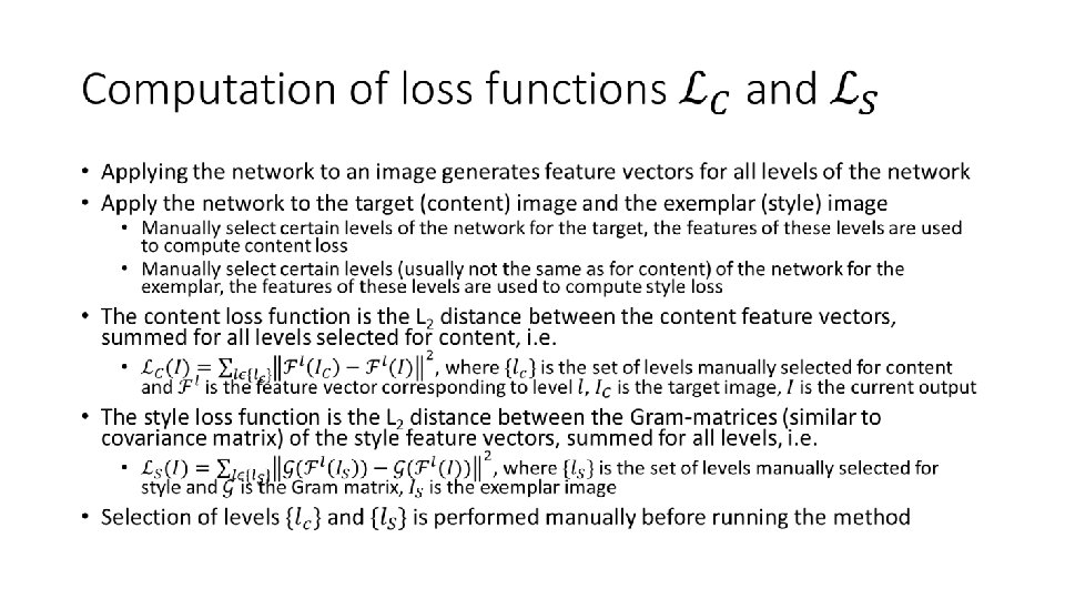
 image Features Exemplar (Style) image Features Features Content loss Features Style")
Levels Target (Content) image Features Exemplar (Style) image Features Features Content loss Features Style loss Result Features Features

Alternative loss functions •

Example results • Results from Gatys, Leon A. , Alexander S. Ecker, and Matthias Bethge. "A neural algorithm of artistic style. " ar. Xiv preprint ar. Xiv: 1508. 06576(2015). • Note that color, texture and shapes are also transferred

Trained CNNs for a different style • The optimization‐based method we have just seen is very slow • Once we have some results for a fixed, single style, we can train a neural network that learns how to apply this particular style • The application (i. e. forward evaluation) of the network is fast (even can be real‐time for videos!), we simply need to send the input through the convoution and pooling layers • Research results showed that we can also train neural networks for a small set of styles it is possible to interpolate between styles

Interpolation between styles

Working examples • AI drawing by NVIDIA: http: //digg. com/video/nvidia‐ai‐drawing • AI fills complete regions with details if the region has a semantic label Video from youtube

Working examples • https: //deepart. io • Browser interface to the first neural network style transfer method • Upload your photo, choose style, wait some minutes and voilá!

Working examples • Collection of links to the implementations of state‐of‐the‐art methods: • https: //github. com/ycjing/Neural‐Style‐Transfer‐Papers • Usually Torch, Tensor. Flow, Caffee or Matlab implementations • Commercial applications based on neural style transfer: • Prisma: https: //prisma‐ai. com • Ostagram: https: //www. ostagram. me
- Slides: 59