Study of the electron identification algorithms in TRD

Study of the electron identification algorithms in TRD Andrey Lebedev 1, 3, Semen Lebedev 2, 3, Gennady Ososkov 3 1 Frankfurt University, 2 Giessen University and 3 LIT JINR

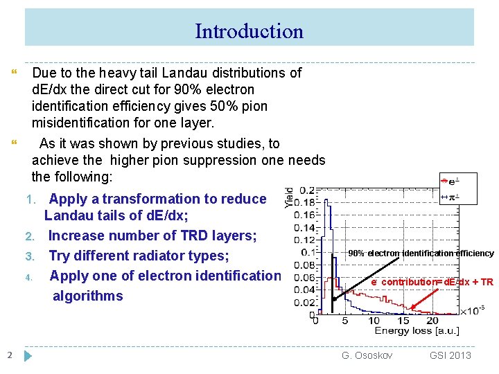
Introduction Due to the heavy tail Landau distributions of d. E/dx the direct cut for 90% electron identification efficiency gives 50% pion misidentification for one layer. As it was shown by previous studies, to achieve the higher pion suppression one needs the following: 1. 2. 3. 4. 2 Apply a transformation to reduce Landau tails of d. E/dx; Increase number of TRD layers; Try different radiator types; Apply one of electron identification algorithms 90% electron identification efficiency e- contribution=d. E/dx + TR G. Ososkov GSI 2013

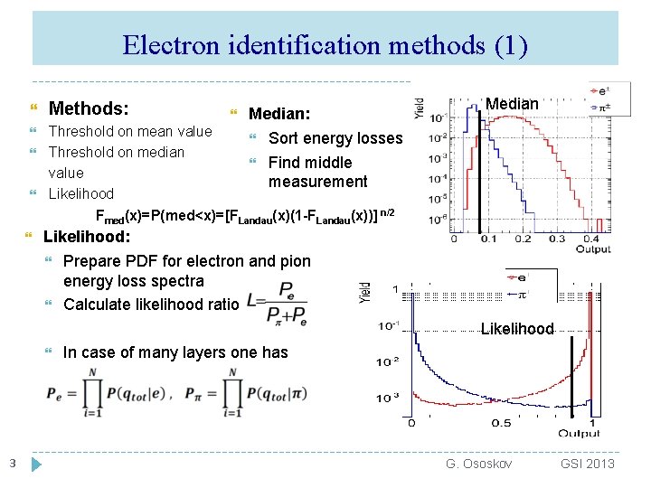
Electron identification methods (1) Methods: Threshold on mean value Threshold on median value Likelihood Fmed(x)=P(med<x)=[FLandau(x)(1 -FLandau(x))] n/2 Median: Sort energy losses Find middle measurement Median Likelihood: Prepare PDF for electron and pion energy loss spectra Calculate likelihood ratio Likelihood 3 In case of many layers one has G. Ososkov GSI 2013

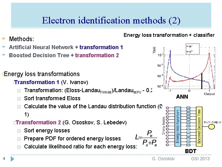
Electron identification methods (2) Methods: Artificial Neural Network + transformation 1 Boosted Decision Tree + transformation 2 � Energy loss transformation + classifier loss transformations � Transformation 1 (V. Ivanov) Transformation: (Eloss-Landau. FWHM)/Landau. MPV - 0. 225 Sort transformed Eloss Calculate the value of the Landau distribution function (0, 1) �Transformation 2 (G. Ososkov, S. Lebedev) Sort energy losses Prepare PDF for ordered energy losses Calculate likelihood ratio for each energy loss: 4 G. Ososkov ANN BDT GSI 2013

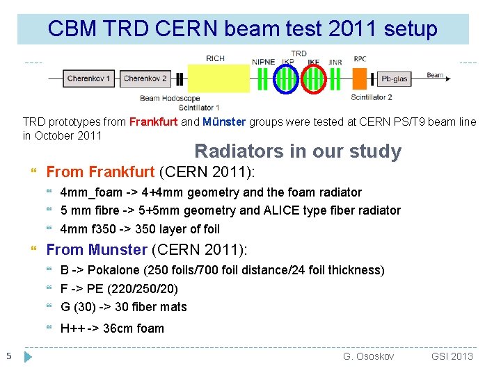
CBM TRD CERN beam test 2011 setup TRD prototypes from Frankfurt and Münster groups were tested at CERN PS/T 9 beam line in October 2011 Radiators in our study From Frankfurt (CERN 2011): From Munster (CERN 2011): B -> Pokalone (250 foils/700 foil distance/24 foil thickness) F -> PE (220/250/20) G (30) -> 30 fiber mats H++ -> 36 cm foam 5 4 mm_foam -> 4+4 mm geometry and the foam radiator 5 mm fibre -> 5+5 mm geometry and ALICE type fiber radiator 4 mm f 350 -> 350 layer of foil G. Ososkov GSI 2013

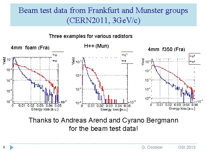
Beam test data from Frankfurt and Munster groups (CERN 2011, 3 Ge. V/c) Three examples for various radistors 4 mm_foam (Fra) H++ (Mun) 4 mm_f 350 (Fra) Thanks to Andreas Arend and Cyrano Bergmann for the beam test data! 6 G. Ososkov GSI 2013

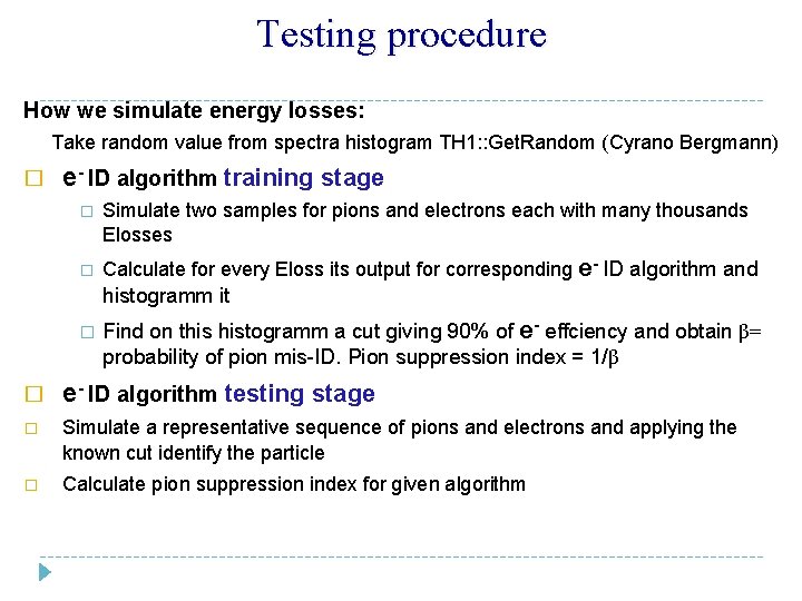
Testing procedure How we simulate energy losses: Take random value from spectra histogram TH 1: : Get. Random (Cyrano Bergmann) � e- ID algorithm training stage � � Simulate two samples for pions and electrons each with many thousands Elosses Calculate for every Eloss its output for corresponding e- ID algorithm and histogramm it � Find on this histogramm a cut giving 90% of e- effciency and obtain β= probability of pion mis-ID. Pion suppression index = 1/β � e- ID algorithm testing stage � Simulate a representative sequence of pions and electrons and applying the known cut identify the particle � Calculate pion suppression index for given algorithm

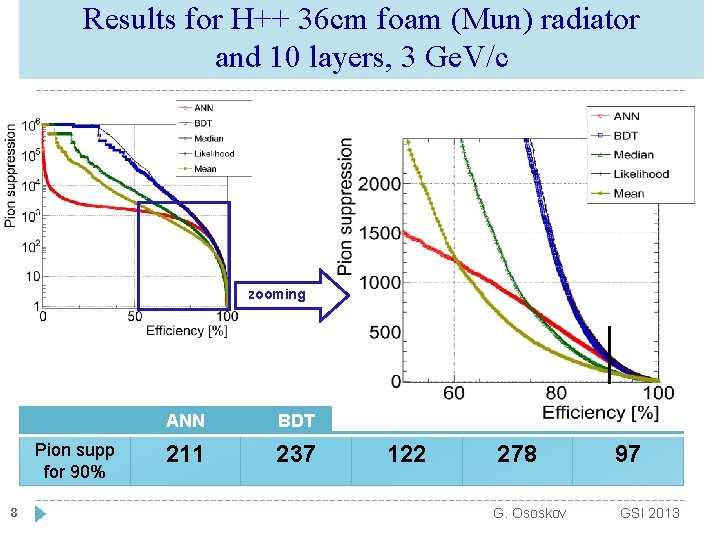
Results for H++ 36 cm foam (Mun) radiator and 10 layers, 3 Ge. V/c zooming Pion supp for 90% 8 ANN BDT Median Likelihood Mean 211 237 122 278 97 G. Ososkov GSI 2013

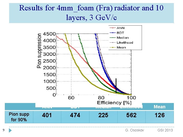
Results for 4 mm_foam (Fra) radiator and 10 layers, 3 Ge. V/c Pion supp for 90% 9 ANN BDT Median Likelihood Mean 401 474 225 562 126 G. Ososkov GSI 2013

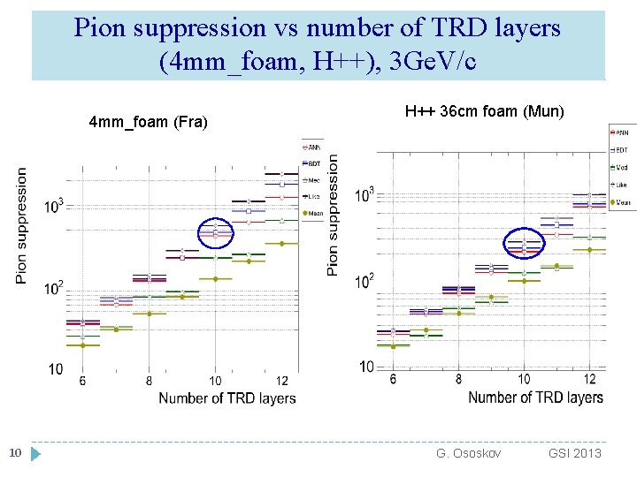
Pion suppression vs number of TRD layers (4 mm_foam, H++), 3 Ge. V/c 4 mm_foam (Fra) 10 H++ 36 cm foam (Mun) G. Ososkov GSI 2013

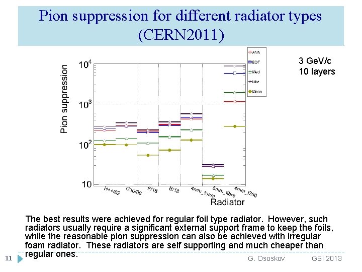
Pion suppression for different radiator types (CERN 2011) 3 Ge. V/c 10 layers 11 The best results were achieved for regular foil type radiator. However, such radiators usually require a significant external support frame to keep the foils, while the reasonable pion suppression can also be achieved with irregular foam radiator. These radiators are self supporting and much cheaper than regular ones. G. Ososkov GSI 2013

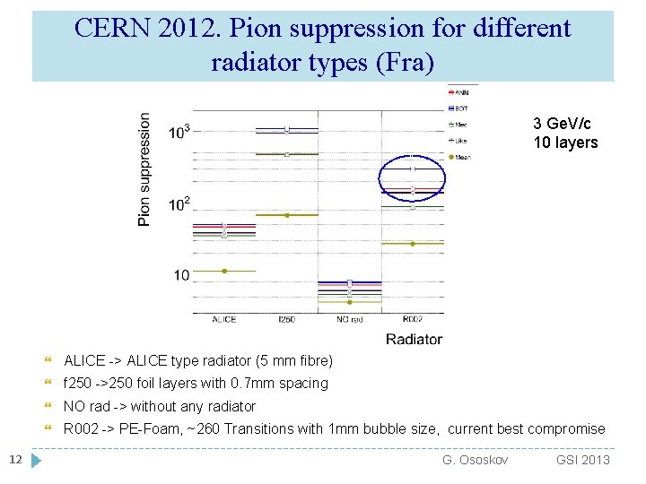
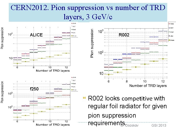
CERN 2012. Pion suppression for different radiator types (Fra) 3 Ge. V/c 10 layers 12 ALICE -> ALICE type radiator (5 mm fibre) f 250 ->250 foil layers with 0. 7 mm spacing NO rad -> without any radiator R 002 -> PE-Foam, ~260 Transitions with 1 mm bubble size, current best compromise G. Ososkov GSI 2013

CERN 2012. Pion suppression vs number of TRD layers, 3 Ge. V/c ALICE R 002 f 250 13 R 002 looks competitive with regular foil radiator for given pion suppression requirements. G. Ososkov GSI 2013

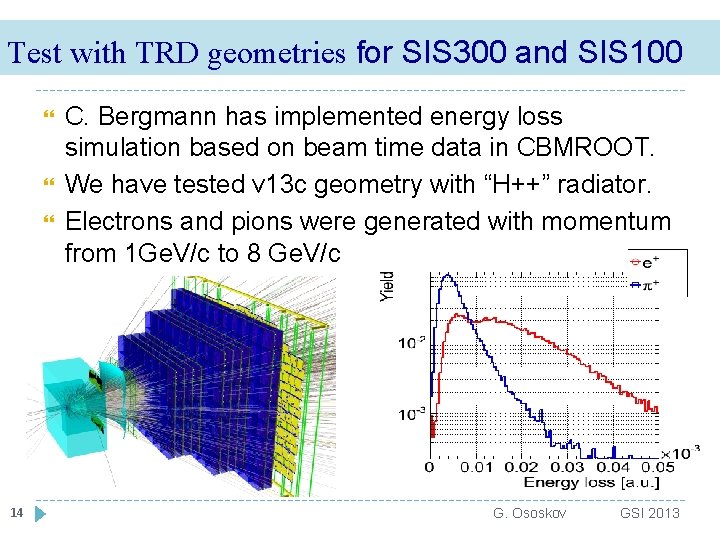
Test with TRD geometries for SIS 300 and SIS 100 14 C. Bergmann has implemented energy loss simulation based on beam time data in CBMROOT. We have tested v 13 c geometry with “H++” radiator. Electrons and pions were generated with momentum from 1 Ge. V/c to 8 Ge. V/c G. Ososkov GSI 2013

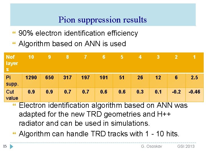
Pion suppression results 90% electron identification efficiency Algorithm based on ANN is used Nof layer s 10 9 8 7 6 5 4 3 2 1 Pi supp. 1290 650 317 197 101 51 26 12 6 2. 5 Cut value 0. 9 0. 7 0. 6 0. 3 0. 1 -0. 2 -0. 46 15 Electron identification algorithm based on ANN was adapted for the new TRD geometries and H++ radiator and can be used in simulations. Algorithm can handle TRD tracks with 1 - 10 hits. G. Ososkov GSI 2013

Summary 16 TRD beam time data from CERN 2011 and 2012 were analyzed with algorithms implemented in CBMROOT. Regular foil type radiator (4 mm_f 350) showed excellent results but extreme difficult to build in large scale. Required pion suppression can also be achieved with irregular foam radiator (H++, 4 mm_foam, R 002) New TRD geometries for SIS 300 and SIS 100 were checked and showed good performance. G. Ososkov GSI 2013

Thanks for your attention! 17

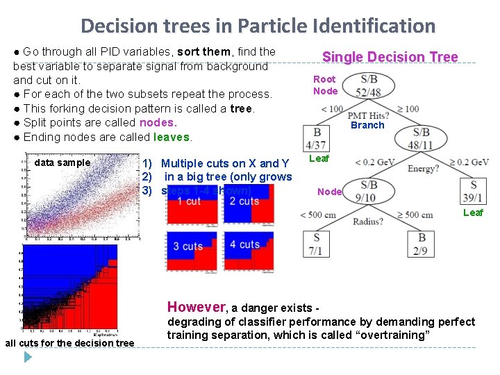
Decision trees in Particle Identification ● Go through all PID variables, sort them, find the best variable to separate signal from background and cut on it. ● For each of the two subsets repeat the process. ● This forking decision pattern is called a tree. ● Split points are called nodes. ● Ending nodes are called leaves. data sample 1) Multiple cuts on X and Y 2) in a big tree (only grows 3) steps 1 -4 shown) Single Decision Tree Root Node Branch Leaf Node Leaf However, a danger exists all cuts for the decision tree degrading of classifier performance by demanding perfect training separation, which is called “overtraining”

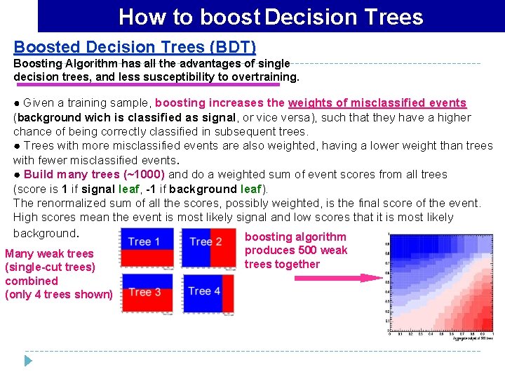
How to boost Decision Trees Boosted Decision Trees (BDT) Boosting Algorithm has all the advantages of single decision trees, and less susceptibility to overtraining. ● Given a training sample, boosting increases the weights of misclassified events (background wich is classified as signal, or vice versa), such that they have a higher chance of being correctly classified in subsequent trees. ● Trees with more misclassified events are also weighted, having a lower weight than trees with fewer misclassified events. ● Build many trees (~1000) and do a weighted sum of event scores from all trees (score is 1 if signal leaf, -1 if background leaf). The renormalized sum of all the scores, possibly weighted, is the final score of the event. High scores mean the event is most likely signal and low scores that it is most likely background. boosting algorithm Many weak trees (single-cut trees) combined (only 4 trees shown) produces 500 weak trees together

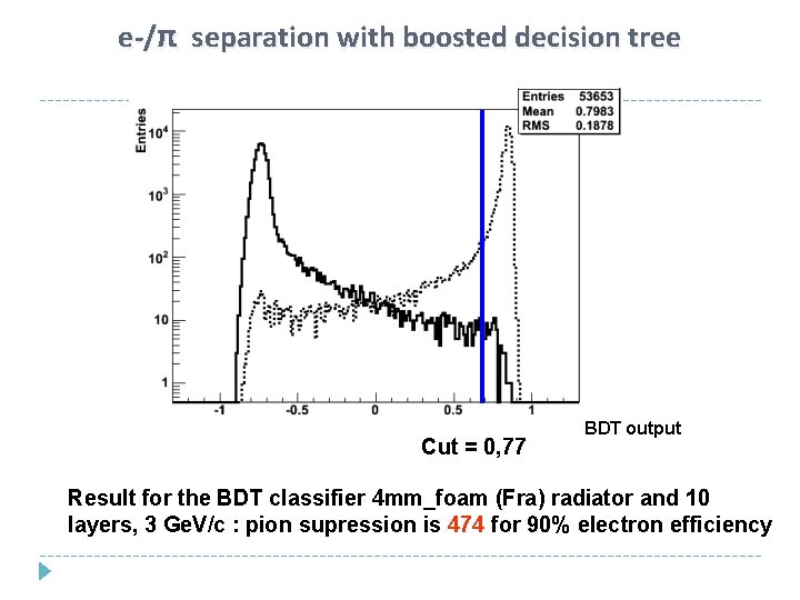
e-/π separation with boosted decision tree Cut = 0, 77 BDT output Result for the BDT classifier 4 mm_foam (Fra) radiator and 10 layers, 3 Ge. V/c : pion supression is 474 for 90% electron efficiency