Students t test l This test was invented

Student’s t test l This test was invented by a statistician working for the brewer Guinness. He was called WS Gosset (1867 -1937), but preferred to keep anonymous so wrote under the name “Student”.

The t-distribution William Gosset lived from 1876 to 1937 Gosset invented the t -test to handle small samples for quality control in brewing. He wrote under the name "Student".

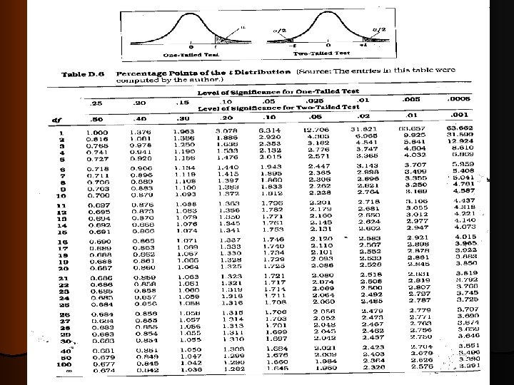
t-Statistic l When the sampled population is normally distributed, the t statistic is Student t distributed with n-1 degrees of freedom.

T-test 1. Test for single mean 2. Whether the sample mean is equal to the predefined population mean ? 3. 4. 2. Test for difference in means 5. Whether the CD 4 level of patients taking treatment A is equal to CD 4 level of patients taking treatment B ? 6. 7. 3. Test for paired observation 8. Whether the treatment conferred any significant benefit ? 9.

T- test for single mean The following are the weight (mg) of each of 20 rats drawn at random from a large stock. Is it likely that the mean weight for the whole stock could be 24 mg, a value observed in some previous work? . 9 14 15 15 16 16 18 18 19 19 20 21 22 22 24 24 26 27 29 30 32

Steps for test for single mean 1. Questioned to be answered 2. Is the Mean weight of the sample of 20 rats is 24 mg? 3. N=20, =21. 0 mg, sd=5. 91 , =24. 0 mg 4. 2. Null Hypothesis 5. The mean weight of rats is 24 mg. That is, The sample mean is equal to population mean. 6. 3. Test statistics 7. 4. 8. 9. --- t (n-1) df Comparison with theoretical value if tab t (n-1) < cal t (n-1) reject Ho, if tab t (n-1) > cal t (n-1) accept Ho,

t –test for single mean l Test statistics n=20, =21. 0 mg, =24. 0 mg t = t. 05, 19 = 2. 093 Inference : sd=5. 91 , Accept H 0 if t < 2. 093 Reject H 0 if t >= 2. 093 There is no evidence that the sample is taken from the population with mean weight of 24 gm

Determining the p-Value Area =. 025 Area =. 005 0 1. 96 2. 575 -1. 96 Area =. 005 Z

f(t). 025 -1. 96 . 95 0 . 025 1. 96 t red area = rejection region for 2 -sided test

T-test for difference in means Given below are the 24 hrs total energy expenditure (MJ/day) in groups of lean and obese women. Examine whether the obese women’s mean energy expenditure is significantly higher ? . Lean 6. 1 7. 5 7. 9 8. 1 10. 9 7. 0 7. 5 5. 5 7. 6 8. 1 8. 4 10. 2 8. 8 9. 7 11. 5 Obese 9. 2 9. 7 11. 8 9. 2 10. 0 12. 8

Two sample t-test Difference between means Sample size Variability of data + + t-test t

T-test for difference in means Null Hypothesis Obese women’s mean energy expenditure is equal to the lean women’s energy expenditure. Test statistics : t(n 1+n 2 -2) 1, 2 - means of sample 1 and sample 2 1, 2 – sd of sample 1 and sample 2 n 1 , n 2 – number of study subjects in sample 1 and sample 2

T-test for difference in means N S Data Summary lean Obese 13 9 8. 10 10. 30 1. 38 1. 25 tab t 9+13 -2 =20 df = t 0. 05, 20 =2. 086 Inference : The cal t (3. 82) is higher than tab t at 0. 05, 20. ie 2. 086. This implies that there is a evidence that the mean energy expenditure in obese group is significantly (p<0. 05) higher than that of lean group

Example Suppose we want to test the effectiveness of a program designed to increase scores on the quantitative section of the Graduate Record Exam (GRE). We test the program on a group of 8 students. Prior to entering the program, each student takes a practice quantitative GRE; after completing the program, each student takes another practice exam. Based on their performance, was the program effective?

l Each subject contributes 2 scores: repeated measures design Student Before Program After Program 1 520 555 2 490 510 3 600 585 4 620 645 5 580 630 6 560 550 7 610 645 8 480 520

l Can represent each student with a single score: the difference (D) between the scores Before Program After Program Student D 1 520 555 35 2 490 510 20 3 600 585 -15 4 620 645 25 5 580 630 50 6 560 550 -10 7 610 645 35 8 480 520 40

l Approach: test the effectiveness of program by testing significance of D l Alternative hypothesis: program is effective → scores after program will be higher than scores before program → average D will be greater than zero H 0 : µ D ≤ 0 H 1 : µ D > 0

So, need to know ∑D and ∑D 2: Student Before Program After Program D D 2 1 520 555 35 1225 2 490 510 20 400 3 600 585 -15 225 4 620 645 25 625 5 580 630 50 2500 6 560 550 -10 100 7 610 645 35 1225 8 480 520 40 1600 ∑D = 180 ∑D 2 = 7900

Recall that for single samples: For related samples: where: and

Mean of D: Standard deviation of D: Standard error:

Under H 0, µD = 0, so: From Table B. 2: for α = 0. 05, one-tailed, with df = 7, tcrit = 1. 895 2. 714 > 1. 895 → reject H 0 The program is effective.

t-Value t is a measure of: How difficult is it to believe the null hypothesis? High t Difficult to believe the null hypothesis accept that there is a real difference. Low t Easy to believe the null hypothesis have not proved any difference.

In Conclusion ! Student ‘s t-test will be used: --- When Sample size is small and for the following situations: (1) to compare the single sample mean with the population mean (2) to compare the sample means of two indpendent samples (3) to compare the sample means of paired samples l