STT 200 LECTURE 5 SECTION 23 24 RECITATION

STT 200 – LECTURE 5, SECTION 23, 24 RECITATION 12 (4/2/2013) TA: Zhen Zhang zhangz 19@stt. msu. edu Office hour: (C 500 WH) 3 -4 PM Tuesday (office tel. : 432 -3342) Help-room: (A 102 WH) 9: 00 AM-1: 00 PM, Monday 1 Class meet on Tuesday: 12: 40 – 1: 30 PM A 224 WH, Section 23 1: 50 – 2: 40 PM A 234 WH, Section 24

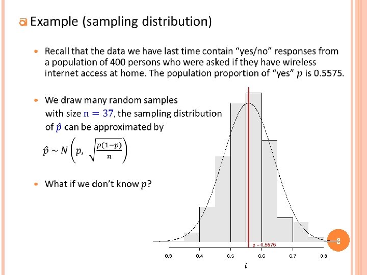
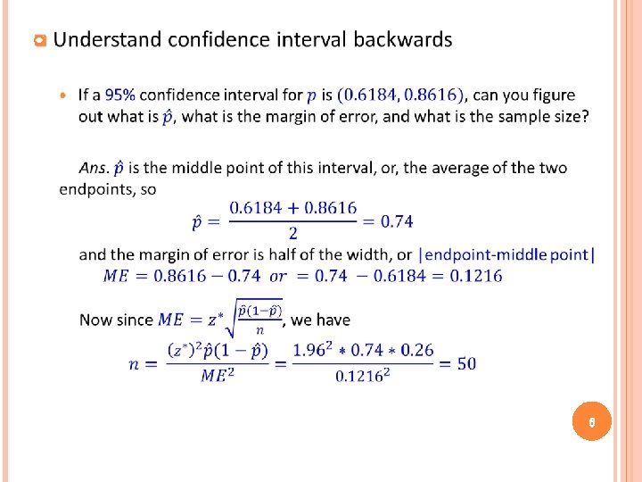
2

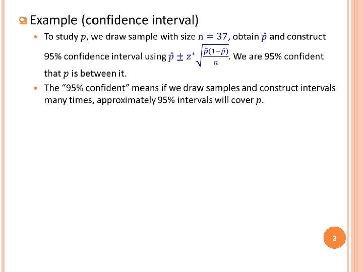
3

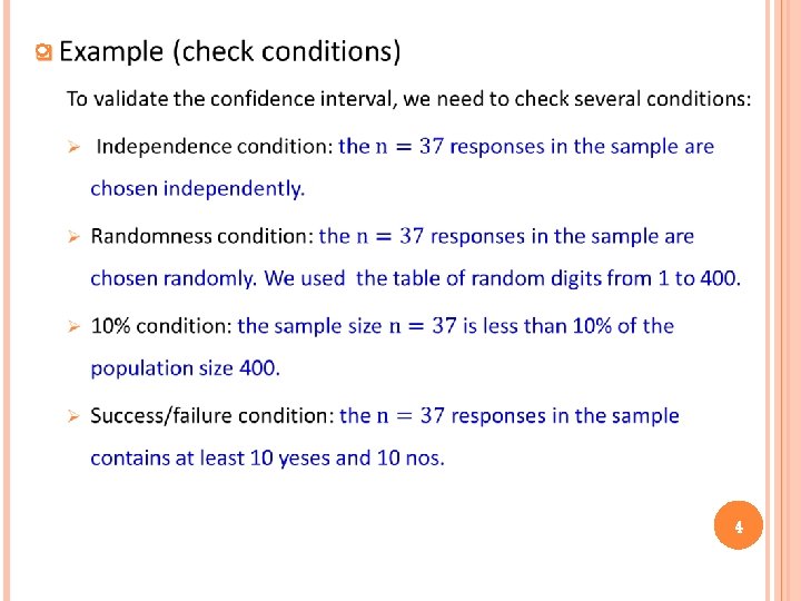
4

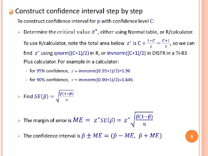
5

6

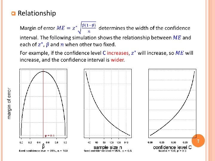
7

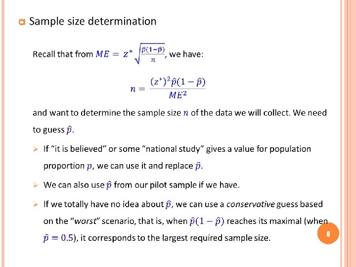
8

NEED SOME COFFEE? 9

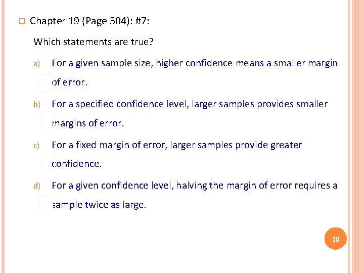
q Chapter 19 (Page 504): #7: Which statements are true? a) For a given sample size, higher confidence means a smaller margin of error. b) For a specified confidence level, larger samples provides smaller margins of error. c) For a fixed margin of error, larger samples provide greater confidence. d) For a given confidence level, halving the margin of error requires a sample twice as large. 10

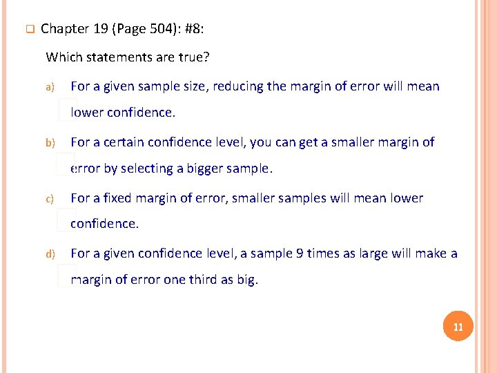
q Chapter 19 (Page 504): #8: Which statements are true? a) For a given sample size, reducing the margin of error will mean lower confidence. b) For a certain confidence level, you can get a smaller margin of error by selecting a bigger sample. c) For a fixed margin of error, smaller samples will mean lower confidence. d) For a given confidence level, a sample 9 times as large will make a margin of error one third as big. 11

12

13

14

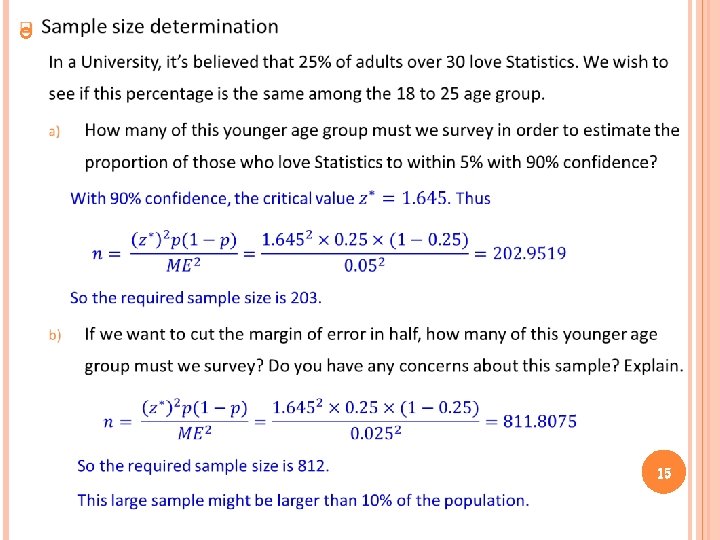
15

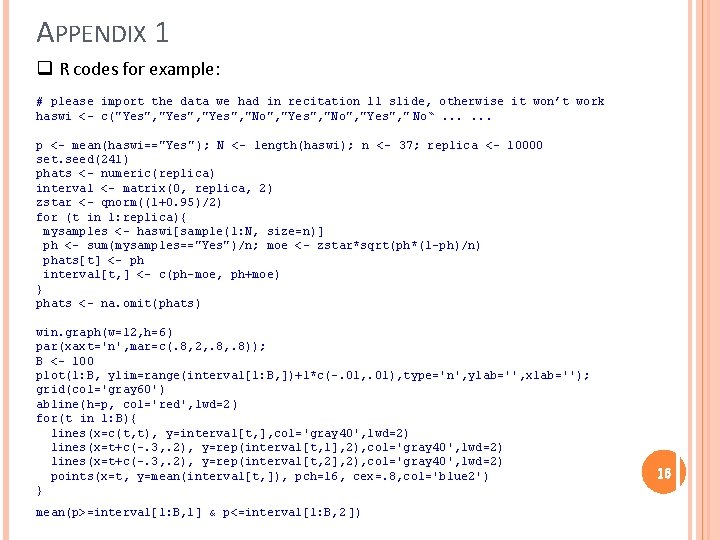
APPENDIX 1 q R codes for example: # please import the data we had in recitation 11 slide, otherwise it won’t work haswi <- c("Yes", "No", "Yes", " No“. . . p <- mean(haswi=="Yes"); N <- length(haswi); n <- 37; replica <- 10000 set. seed(241) phats <- numeric(replica) interval <- matrix(0, replica, 2) zstar <- qnorm((1+0. 95)/2) for (t in 1: replica){ mysamples <- haswi[sample(1: N, size=n)] ph <- sum(mysamples=="Yes")/n; moe <- zstar*sqrt(ph*(1 -ph)/n) phats[t] <- ph interval[t, ] <- c(ph-moe, ph+moe) } phats <- na. omit(phats) win. graph(w=12, h=6) par(xaxt='n', mar=c(. 8, 2, . 8)); B <- 100 plot(1: B, ylim=range(interval[1: B, ])+1*c(-. 01, . 01), type='n', ylab='', xlab=''); grid(col='gray 60') abline(h=p, col='red', lwd=2 ) for(t in 1: B){ lines(x=c(t, t), y=interval[t, ], col='gray 40', lwd=2) lines(x=t+c(-. 3, . 2), y=rep(interval[t, 1], 2), col='gray 40', lwd=2) lines(x=t+c(-. 3, . 2), y=rep(interval[t, 2], 2), col='gray 40', lwd=2) points(x=t, y=mean(interval[t, ]), pch=16, cex=. 8, col='blue 2') } mean(p>=interval[1: B, 1] & p<=interval[1: B, 2 ]) 16

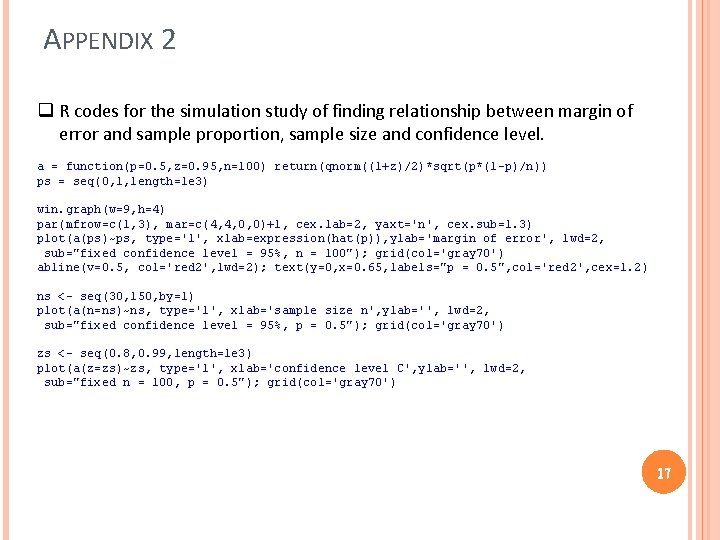
APPENDIX 2 q R codes for the simulation study of finding relationship between margin of error and sample proportion, sample size and confidence level. a = function(p=0. 5, z=0. 95, n=100) return(qnorm((1+z)/2)*sqrt(p*(1 -p)/n)) ps = seq(0, 1, length=1 e 3) win. graph(w=9, h=4) par(mfrow=c(1, 3), mar=c(4, 4, 0, 0)+1, cex. lab=2, yaxt='n', cex. sub=1. 3) plot(a(ps)~ps, type='l', xlab=expression(hat(p)), ylab='margin of error', lwd=2, sub="fixed confidence level = 95%, n = 100"); grid(col='gray 70') abline(v=0. 5, col='red 2', lwd=2); text(y=0, x=0. 65, labels="p = 0. 5", col='red 2', cex=1. 2) ns <- seq(30, 150, by=1) plot(a(n=ns)~ns, type='l', xlab='sample size n', ylab='', lwd=2, sub="fixed confidence level = 95%, p = 0. 5"); grid(col='gray 70') zs <- seq(0. 8, 0. 99, length=1 e 3) plot(a(z=zs)~zs, type='l', xlab='confidence level C', ylab='', lwd=2, sub="fixed n = 100, p = 0. 5"); grid(col='gray 70') 17

Thank you. 18