Structural Equation Modeling l SEM an entire family

Structural Equation Modeling l SEM, an entire family of models known by many names Covariance structure analysis – Latent variable analysis – Confirmatory factor analysis – LISREL analysis – l Combination of econometrics and measurement from psychological and sociology Fall, 2008 Multivariate Analysis Lec 10 1

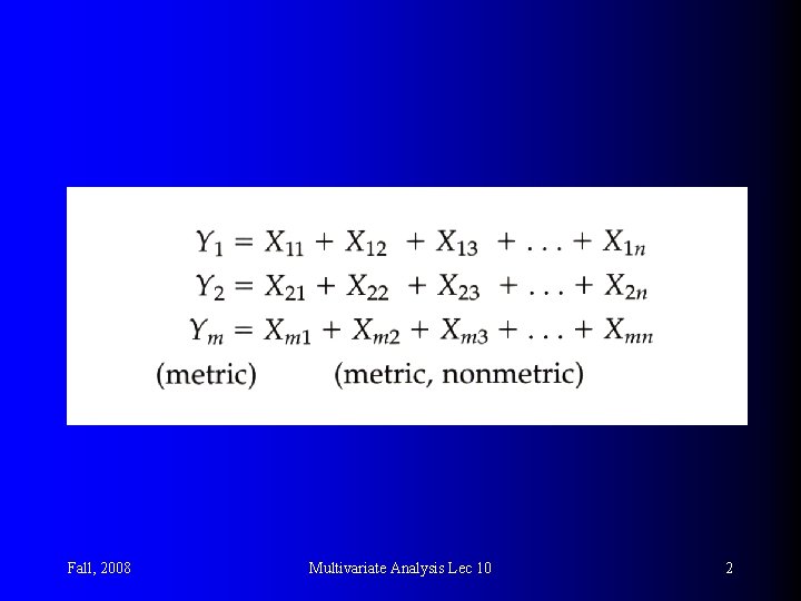
Fall, 2008 Multivariate Analysis Lec 10 2

l Three distinguishing characteristics: – Estimation of multiple and interrelated dependence relationships l – The structural model (a series of structural equations, similar to regression equations) The ability to represent unobserved concepts and account for measurement error in the estimation process Latent variables: a hypothetical and unobserved concept that can only be approximated by observable variables l manifested variables: the observed variables l Sound like a nonsensical approach? l – Fall, 2008 Defining a model to explain the entire set of relationships Multivariate Analysis Lec 10 3

l Benefits of Using Latent Constructs – Improving statistical estimation l l l The “true” or structural coefficient between DV & IV The reliability of predictor variable Reliability and measurement error Regression coefficient: y. x= s x All dependence relationships are based on the observed correlation – Representing theoretical concepts l l Unsure how to answer the questions Interpret the questions differently – Specifying measurement error l Fall, 2008 Measurement model Multivariate Analysis Lec 10 4

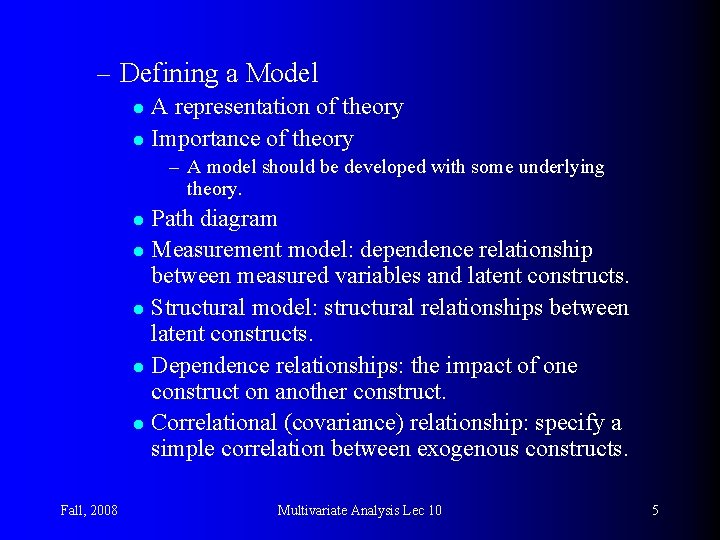
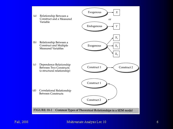
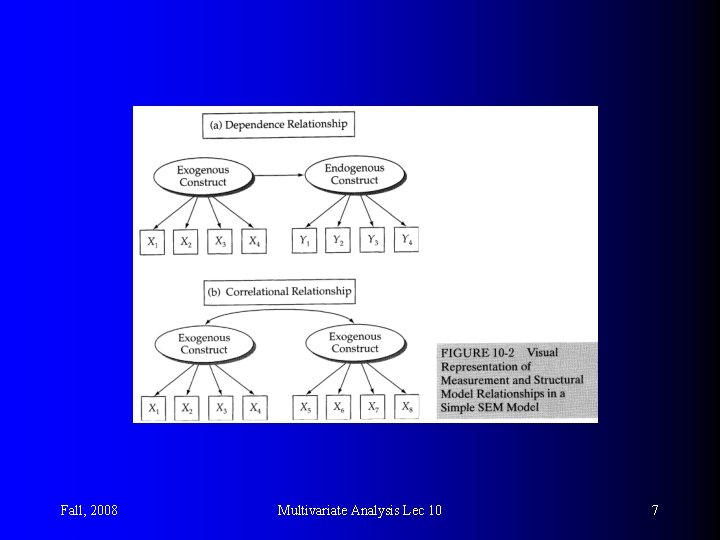
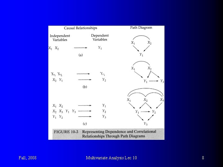
– Defining a Model A representation of theory l Importance of theory l – A model should be developed with some underlying theory. Path diagram l Measurement model: dependence relationship between measured variables and latent constructs. l Structural model: structural relationships between latent constructs. l Dependence relationships: the impact of one construct on another construct. l Correlational (covariance) relationship: specify a simple correlation between exogenous constructs. l Fall, 2008 Multivariate Analysis Lec 10 5

Fall, 2008 Multivariate Analysis Lec 10 6

Fall, 2008 Multivariate Analysis Lec 10 7

Fall, 2008 Multivariate Analysis Lec 10 8

SEM and Other Multivariate Techniques l SEM is most appropriate when – The research has multiple constructs. – Each construct is represented by several measured variables. – These constructs are distinguished based on whether they are exogenous or endogenous. l SEM shows similarity to other dependence multivariate techniques l The measurement models looks similar to factor analysis Fall, 2008 Multivariate Analysis Lec 10 9

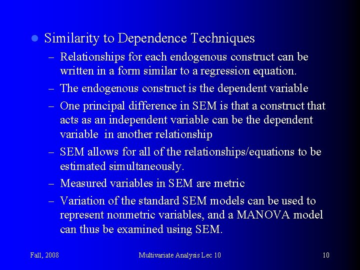
l Similarity to Dependence Techniques – Relationships for each endogenous construct can be – – – Fall, 2008 written in a form similar to a regression equation. The endogenous construct is the dependent variable One principal difference in SEM is that a construct that acts as an independent variable can be the dependent variable in another relationship SEM allows for all of the relationships/equations to be estimated simultaneously. Measured variables in SEM are metric Variation of the standard SEM models can be used to represent nonmetric variables, and a MANOVA model can thus be examined using SEM. Multivariate Analysis Lec 10 10

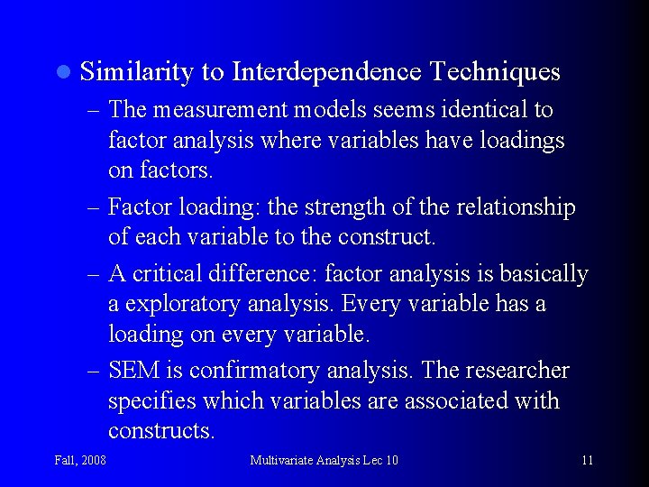
l Similarity to Interdependence Techniques – The measurement models seems identical to factor analysis where variables have loadings on factors. – Factor loading: the strength of the relationship of each variable to the construct. – A critical difference: factor analysis is basically a exploratory analysis. Every variable has a loading on every variable. – SEM is confirmatory analysis. The researcher specifies which variables are associated with constructs. Fall, 2008 Multivariate Analysis Lec 10 11

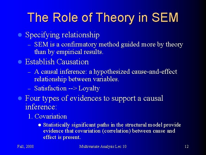
The Role of Theory in SEM l Specifying relationship – l SEM is a confirmatory method guided more by theory than by empirical results. Establish Causation A causal inference: a hypothesized cause-and-effect relationship between variables. – Satisfaction --> Loyalty – l Four types of evidences to support a causal inference: 1. Covariation l Fall, 2008 Statistically significant paths in the structural model provide evidence that covariation (correlation) between cause and effect is present. Multivariate Analysis Lec 10 12

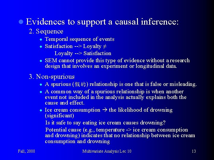
l Evidences to support a causal inference: 2. Sequence l l l Temporal sequence of events Satisfaction --> Loyalty ≠ Loyalty --> Satisfaction SEM cannot provide this type of evidence without a research design that involves an experiment or longitudinal data. 3. Non-spurious l l l Fall, 2008 A spurious (假的) relationship is one that is false or misleading. A common way of a spurious relationship is when another event not included in the analysis actually explains both the cause and effect. Ice cream consumption the likelihood of drowning (significant) Is it safe to say eating ice cream causes drowning? Potential cause (e. g. , temperature -> ice cream consumption and drowning) indicates that no relationship between ice cream consumption and drowning Multivariate Analysis Lec 10 13

l Conditions with No Collinearity – Causal evidence is most easily presented when the set of predictors for some effect is unrelated to one another. – When collinearity is not present, the researcher comes closest to reproducing the conditions in an experimental design. – These conditions include orthogonal, or uncorrelated, experimental predictor variables. l Conditions with Multicollinearity – Often the predictor variables show some relationships with other predictors and the effect construct making a causal inference less certain. Fall, 2008 Multivariate Analysis Lec 10 14

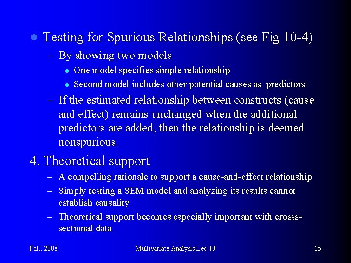
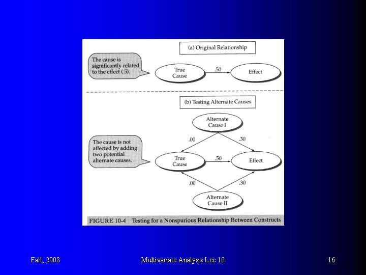
l Testing for Spurious Relationships (see Fig 10 -4) – By showing two models l l One model specifies simple relationship Second model includes other potential causes as predictors – If the estimated relationship between constructs (cause and effect) remains unchanged when the additional predictors are added, then the relationship is deemed nonspurious. 4. Theoretical support – A compelling rationale to support a cause-and-effect relationship – Simply testing a SEM model and analyzing its results cannot establish causality – Theoretical support becomes especially important with crossssectional data Fall, 2008 Multivariate Analysis Lec 10 15

Fall, 2008 Multivariate Analysis Lec 10 16

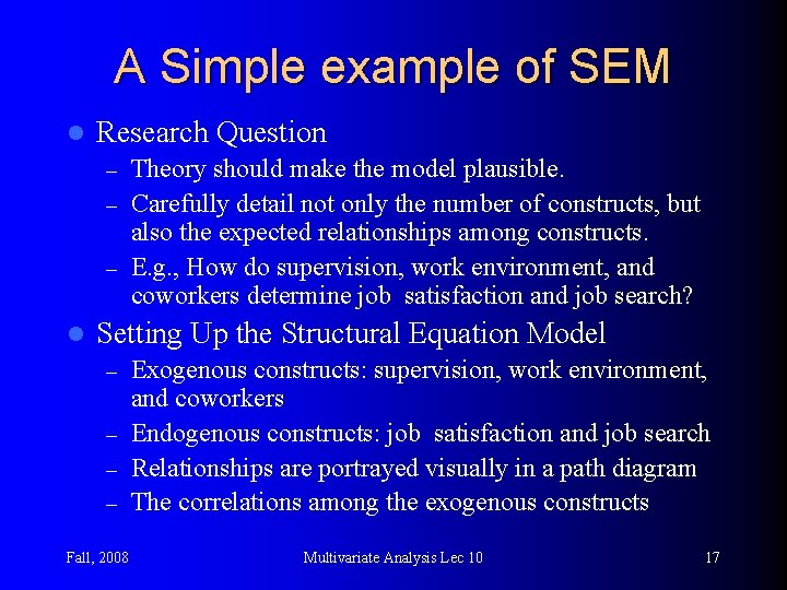
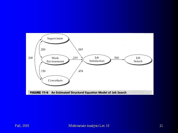
A Simple example of SEM l Research Question Theory should make the model plausible. – Carefully detail not only the number of constructs, but also the expected relationships among constructs. – E. g. , How do supervision, work environment, and coworkers determine job satisfaction and job search? – l Setting Up the Structural Equation Model Exogenous constructs: supervision, work environment, and coworkers – Endogenous constructs: job satisfaction and job search – Relationships are portrayed visually in a path diagram – The correlations among the exogenous constructs – Fall, 2008 Multivariate Analysis Lec 10 17

Fall, 2008 Multivariate Analysis Lec 10 18

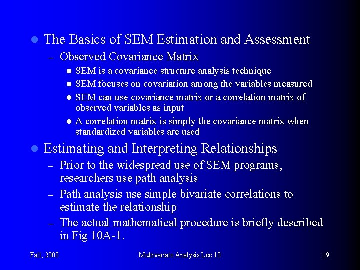
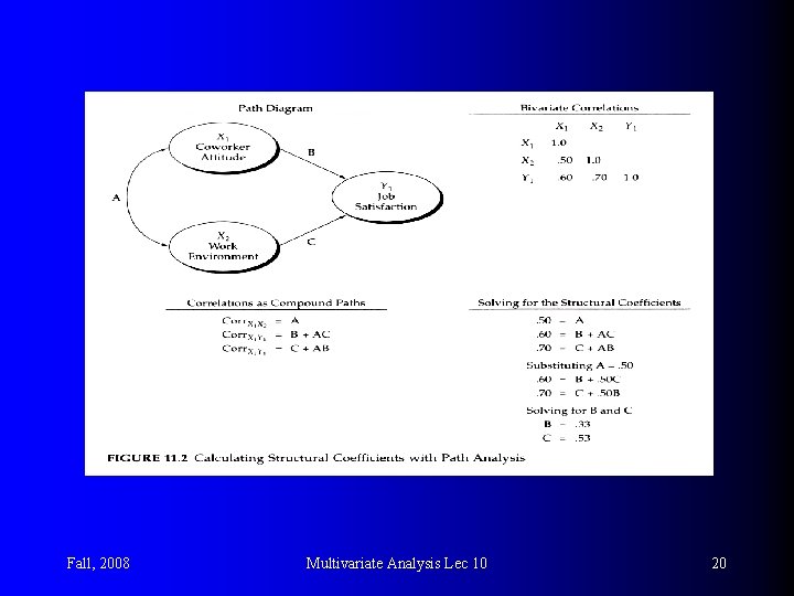
l The Basics of SEM Estimation and Assessment – Observed Covariance Matrix SEM is a covariance structure analysis technique l SEM focuses on covariation among the variables measured l SEM can use covariance matrix or a correlation matrix of observed variables as input l A correlation matrix is simply the covariance matrix when standardized variables are used l l Estimating and Interpreting Relationships Prior to the widespread use of SEM programs, researchers use path analysis – Path analysis use simple bivariate correlations to estimate the relationship – The actual mathematical procedure is briefly described in Fig 10 A-1. – Fall, 2008 Multivariate Analysis Lec 10 19

Fall, 2008 Multivariate Analysis Lec 10 20

Fall, 2008 Multivariate Analysis Lec 10 21

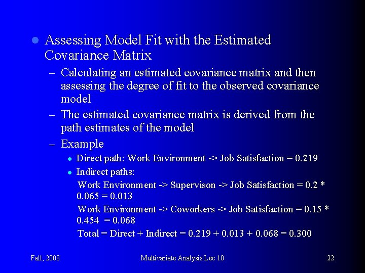
l Assessing Model Fit with the Estimated Covariance Matrix – Calculating an estimated covariance matrix and then assessing the degree of fit to the observed covariance model – The estimated covariance matrix is derived from the path estimates of the model – Example l l Fall, 2008 Direct path: Work Environment -> Job Satisfaction = 0. 219 Indirect paths: Work Environment -> Supervison -> Job Satisfaction = 0. 2 * 0. 065 = 0. 013 Work Environment -> Coworkers -> Job Satisfaction = 0. 15 * 0. 454 = 0. 068 Total = Direct + Indirect = 0. 219 + 0. 013 + 0. 068 = 0. 300 Multivariate Analysis Lec 10 22

l The difference between the observed and estimated covariance matrices become the key driver in assessing the fit of a SEM model Fall, 2008 Multivariate Analysis Lec 10 23

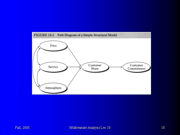
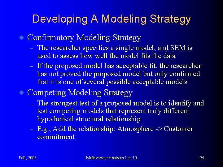
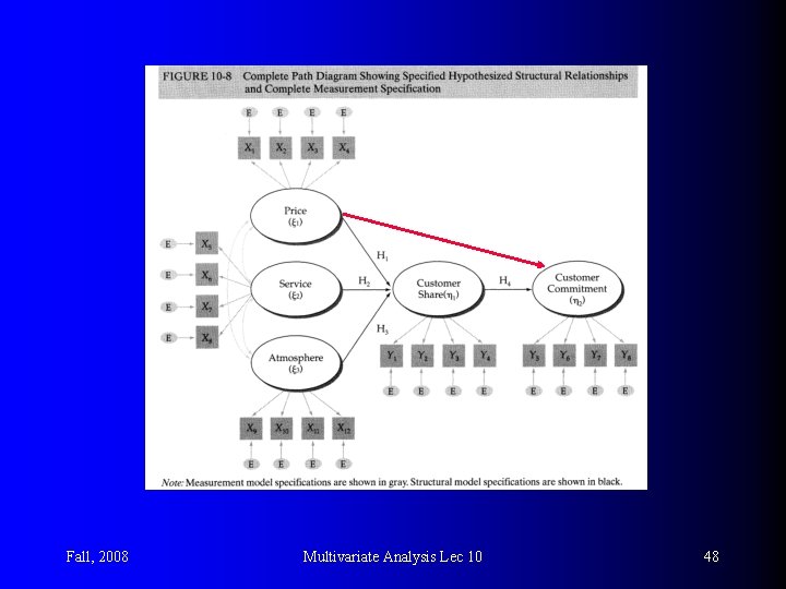
Developing A Modeling Strategy l Confirmatory Modeling Strategy The researcher specifies a single model, and SEM is used to assess how well the model fits the data – If the proposed model has acceptable fit, the researcher has not proved the proposed model but only confirmed that it is one of several possible acceptable models – l Competing Modeling Strategy The strongest test of a proposed model is to identify and test competing models that represent truly different hypothetical structural relationship – E. g. , Add the relationship: Atmosphere -> Customer commitment – Fall, 2008 Multivariate Analysis Lec 10 24

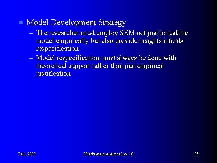
l Model Development Strategy – The researcher must employ SEM not just to test the model empirically but also provide insights into its respecification – Model respecification must always be done with theoretical support rather than just empirical justification Fall, 2008 Multivariate Analysis Lec 10 25

Six Stages in SEM 1. Defining individual constructs 2. Developing the overall measurement model 3. Designing a study to produce empirical results 4. Assessing the measurement model validity 5. Specifying the structural model 6. Assessing structural model validity Fall, 2008 Multivariate Analysis Lec 10 26

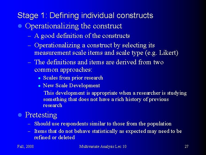
Stage 1: Defining individual constructs l Operationalizing the construct – A good definition of the constructs – Operationalizing a construct by selecting its measurement scale items and scale type (e. g. Likert) – The definitions and items are derived from two common approaches: l l l Scales from prior research New Scale Development This development is appropriate when a researcher is studying something that does not have a rich history of previous research Pretesting – Should use respondents similar to those from the population – Items that do not behave statistically as expected may need to be refined or deleted Fall, 2008 Multivariate Analysis Lec 10 27

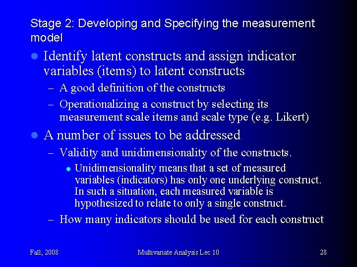
Stage 2: Developing and Specifying the measurement model l Identify latent constructs and assign indicator variables (items) to latent constructs – A good definition of the constructs – Operationalizing a construct by selecting its measurement scale items and scale type (e. g. Likert) l A number of issues to be addressed – Validity and unidimensionality of the constructs. l Unidimensionality means that a set of measured variables (indicators) has only one underlying construct. In such a situation, each measured variable is hypothesized to relate to only a single construct. – How many indicators should be used for each construct Fall, 2008 Multivariate Analysis Lec 10 28

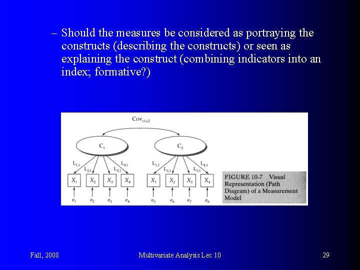
– Should the measures be considered as portraying the constructs (describing the constructs) or seen as explaining the construct (combining indicators into an index; formative? ) Fall, 2008 Multivariate Analysis Lec 10 29

Stage 3: Designing a study to produce empirical results l Research design – Type of data analyzed: covariance or correlation – Missing data – Sample size l Model Estimation – Model structure – Estimation technique – Computer software used Fall, 2008 Multivariate Analysis Lec 10 30

Issues in Research Design l Covariance vs. correlation SEM was originally developed using covariance matrices Using correlations due to ease of interpretation Most SEM program support raw data Consider choice of correlations vs. covariance primarily based on interpretive and statistical issues – Interpretation l Both correlation and covariance inputs can result in standardized parameter estimates. As such, correlations hold no real advantage over covariances – Statistical impact – – l l Fall, 2008 The advantage of using covariances arise from statistical consideration The use of correlations leads to errors in standard error computations Information about magnitude of values (e. g. , comparing means) is not retained using correlations Any comparisons between samples require that covariances be used as input Multivariate Analysis Lec 10 31

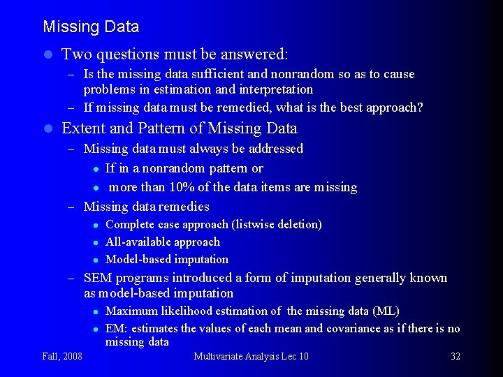
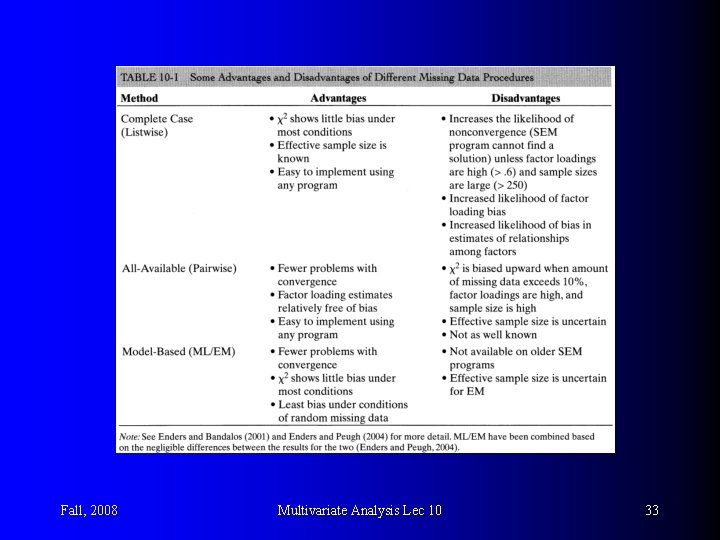
Missing Data l Two questions must be answered: – Is the missing data sufficient and nonrandom so as to cause problems in estimation and interpretation – If missing data must be remedied, what is the best approach? l Extent and Pattern of Missing Data – Missing data must always be addressed If in a nonrandom pattern or l more than 10% of the data items are missing – Missing data remedies l l Complete case approach (listwise deletion) All-available approach Model-based imputation – SEM programs introduced a form of imputation generally known as model-based imputation l l Fall, 2008 Maximum likelihood estimation of the missing data (ML) EM: estimates the values of each mean and covariance as if there is no missing data Multivariate Analysis Lec 10 32

Fall, 2008 Multivariate Analysis Lec 10 33

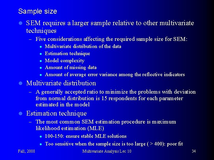
Sample size l SEM requires a larger sample relative to other multivariate techniques – Five considerations affecting the required sample size for SEM: l Multivariate distribution of the data l Estimation technique l Model complexity l Amount of missing data l Amount of average error variance among the reflective indicators l Multivariate distribution – A generally accepted ratio to minimize the problems with deviation from normal distribution is 15 respondents for each parameter estimated in the model l Estimation technique – The most common SEM estimation procedure is maximum likelihood estimation (MLE) l l Fall, 2008 100 -150: ensure stable MLE solutions Too sensitive when the sample size is too large ( > 400): poor fit Multivariate Analysis Lec 10 34

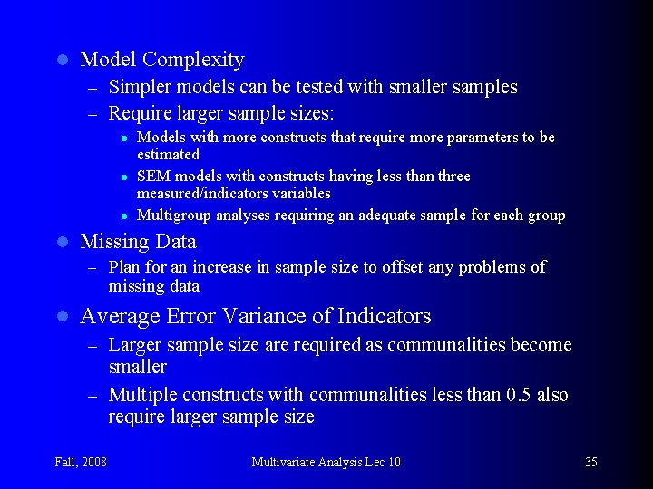
l Model Complexity – Simpler models can be tested with smaller samples – Require larger sample sizes: l l Models with more constructs that require more parameters to be estimated SEM models with constructs having less than three measured/indicators variables Multigroup analyses requiring an adequate sample for each group Missing Data – Plan for an increase in sample size to offset any problems of missing data l Average Error Variance of Indicators – Larger sample size are required as communalities become smaller – Multiple constructs with communalities less than 0. 5 also require larger sample size Fall, 2008 Multivariate Analysis Lec 10 35

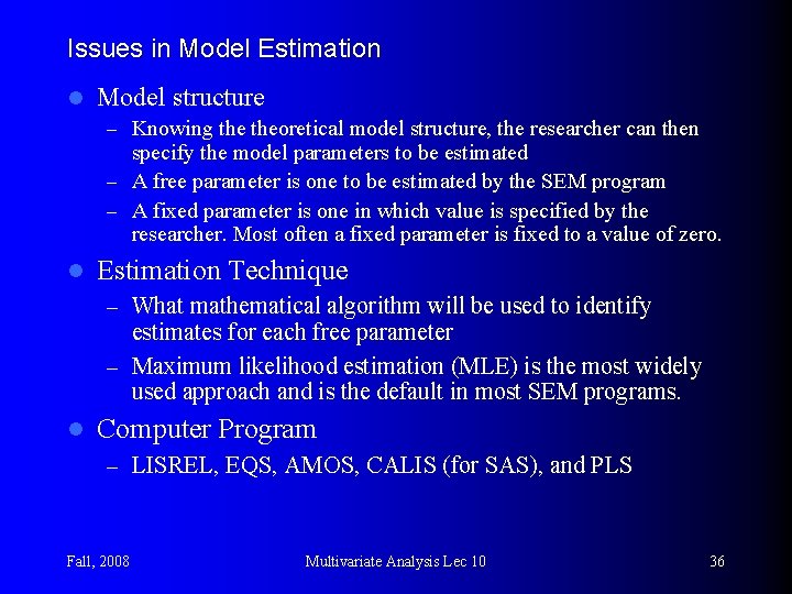
Issues in Model Estimation l Model structure – Knowing theoretical model structure, the researcher can then specify the model parameters to be estimated – A free parameter is one to be estimated by the SEM program – A fixed parameter is one in which value is specified by the researcher. Most often a fixed parameter is fixed to a value of zero. l Estimation Technique – What mathematical algorithm will be used to identify estimates for each free parameter – Maximum likelihood estimation (MLE) is the most widely used approach and is the default in most SEM programs. l Computer Program – LISREL, EQS, AMOS, CALIS (for SAS), and PLS Fall, 2008 Multivariate Analysis Lec 10 36

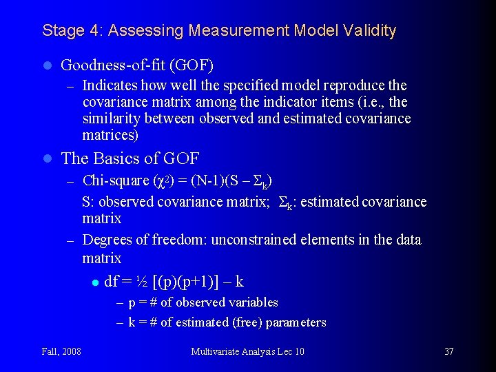
Stage 4: Assessing Measurement Model Validity l Goodness-of-fit (GOF) – Indicates how well the specified model reproduce the covariance matrix among the indicator items (i. e. , the similarity between observed and estimated covariance matrices) l The Basics of GOF – Chi-square (χ2) = (N-1)(S – Σk) S: observed covariance matrix; Σk: estimated covariance matrix – Degrees of freedom: unconstrained elements in the data matrix l df = ½ [(p)(p+1)] – k – p = # of observed variables – k = # of estimated (free) parameters Fall, 2008 Multivariate Analysis Lec 10 37

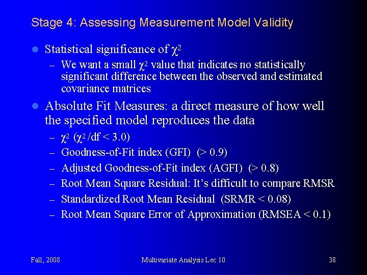
Stage 4: Assessing Measurement Model Validity l Statistical significance of χ2 – We want a small χ2 value that indicates no statistically significant difference between the observed and estimated covariance matrices l Absolute Fit Measures: a direct measure of how well the specified model reproduces the data – χ2 (χ2 /df < 3. 0) – Goodness-of-Fit index (GFI) (> 0. 9) – Adjusted Goodness-of-Fit index (AGFI) (> 0. 8) – Root Mean Square Residual: It’s difficult to compare RMSR – Standardized Root Mean Residual (SRMR < 0. 08) – Root Mean Square Error of Approximation (RMSEA < 0. 1) Fall, 2008 Multivariate Analysis Lec 10 38

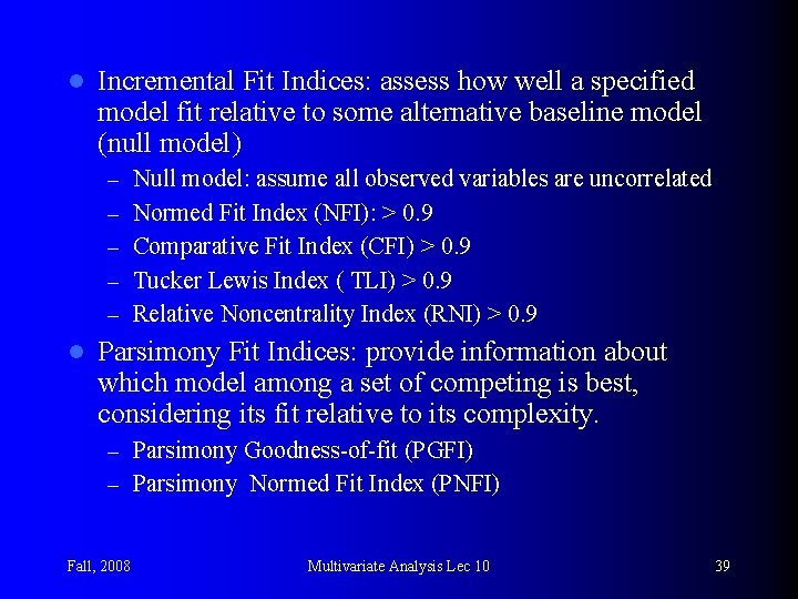
l Incremental Fit Indices: assess how well a specified model fit relative to some alternative baseline model (null model) – Null model: assume all observed variables are uncorrelated – Normed Fit Index (NFI): > 0. 9 – Comparative Fit Index (CFI) > 0. 9 – Tucker Lewis Index ( TLI) > 0. 9 – Relative Noncentrality Index (RNI) > 0. 9 l Parsimony Fit Indices: provide information about which model among a set of competing is best, considering its fit relative to its complexity. – Parsimony Goodness-of-fit (PGFI) – Parsimony Normed Fit Index (PNFI) Fall, 2008 Multivariate Analysis Lec 10 39

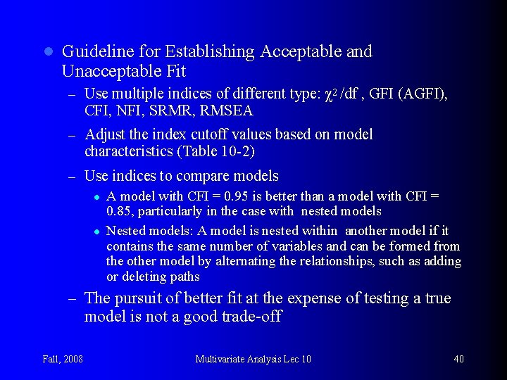
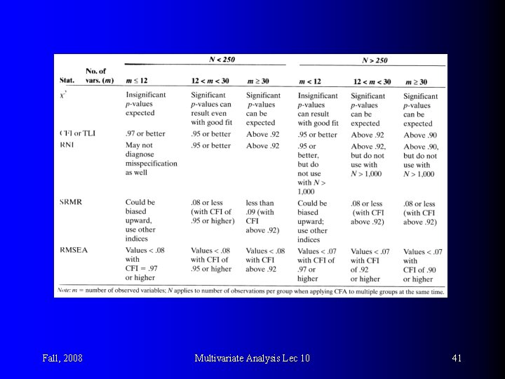
l Guideline for Establishing Acceptable and Unacceptable Fit – Use multiple indices of different type: χ2 /df , GFI (AGFI), CFI, NFI, SRMR, RMSEA – Adjust the index cutoff values based on model characteristics (Table 10 -2) – Use indices to compare models l A model with CFI = 0. 95 is better than a model with CFI = 0. 85, particularly in the case with nested models l Nested models: A model is nested within another model if it contains the same number of variables and can be formed from the other model by alternating the relationships, such as adding or deleting paths – The pursuit of better fit at the expense of testing a true model is not a good trade-off Fall, 2008 Multivariate Analysis Lec 10 40

Fall, 2008 Multivariate Analysis Lec 10 41

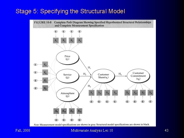
Stage 5: Specifying the Structural Model Specifying the structural model by assigning relationships from one construct to another construct based on the proposed theoretical model. l Each hypothesis represents a specific relationship that must be specified. l Fall, 2008 Multivariate Analysis Lec 10 42

Stage 5: Specifying the Structural Model Fall, 2008 Multivariate Analysis Lec 10 43

Stage 6: Assessing the Structural Model Validity Test validity of the structural model and its corresponding hypothesized theoretical relationships (H 1 ~ H 4). l If the measurement model is validated, then we can perform a valid test of the structural relationships. l Two key differences arising in testing the fit of a structural model relative to measurement model: l – Alternative or competing models can be compared if a competing model approach is taken. – Particular emphasis is placed on the estimated parameters for the structural relationships. Fall, 2008 Multivariate Analysis Lec 10 44

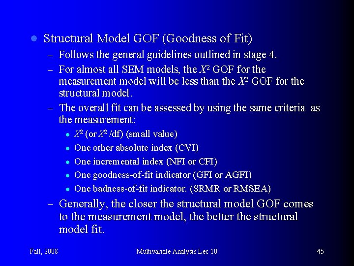
l Structural Model GOF (Goodness of Fit) – Follows the general guidelines outlined in stage 4. – For almost all SEM models, the X 2 GOF for the measurement model will be less than the X 2 GOF for the structural model. – The overall fit can be assessed by using the same criteria as the measurement: l l l X 2 (or X 2 /df) (small value) One other absolute index (CVI) One incremental index (NFI or CFI) One goodness-of-fit indicator (GFI or AGFI) One badness-of-fit indicator. (SRMR or RMSEA) – Generally, the closer the structural model GOF comes to the measurement model, the better the structural model fit. Fall, 2008 Multivariate Analysis Lec 10 45

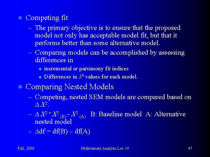
l Competing fit – The primary objective is to ensure that the proposed model not only has acceptable model fit, but that it performs better than some alternative model. – Comparing models can be accomplished by assessing differences in l l l incremental or parsimony fit indices Differences in X 2 values for each model. Comparing Nested Models – Competing, nested SEM models are compared based on ∆ X 2. – ∆ X 2 = X 2 (B) - X 2 (A) B: Baseline model A: Alternative nested model – ∆df = df(B) – df(A) Fall, 2008 Multivariate Analysis Lec 10 46

l Competing fit – The primary objective is to ensure that the proposed model not only has acceptable model fit, but that it performs better than some alternative model. – Comparing models can be accomplished by assessing differences in l l l incremental or parsimony fit indices Differences in X 2 values for each model. Comparing Nested Models – Competing, nested SEM models are compared based on ∆ X 2. – ∆ X 2 = X 2 (B) - X 2 (A) B: Baseline model A: Alternative nested model – ∆df = df(B) – df(A) Fall, 2008 Multivariate Analysis Lec 10 47

Fall, 2008 Multivariate Analysis Lec 10 48

l An example – Adding a path from the Price construct to the Customer Commitment construct. – ∆df = 1 (one additional path) – ∆ X 2 >= 3. 84 would be significant at the 0. 05 level. The researcher would conclude that the alternative model was a significant better fit. – However, theoretical support for the new relationship (new path) is necessary. l Equivalent models – Models with the same estimated covariance matrix. – Even favorable fit statistics are found, other models can provide an equivalent fit Fall, 2008 Multivariate Analysis Lec 10 49

l Testing structural relationships – A theoretical model is considered valid to the extent that the parameter estimates are: l Statistically significant and in the predicted direction. l Nontrivial. This characteristics should be checked using the completely standardized loading estimates (path coefficients). l R 2. Examine the variance explained estimates for the endogenous constructs. Fall, 2008 Multivariate Analysis Lec 10 50