Structural Bioinformatics II Lecture 15 Introduction to Molecular

Structural Bioinformatics II Lecture 15: Introduction to Molecular Dynamics in Drug Design, Part II Dr. Qinfang Sun

Part I: Non-polarizable Non-dissociative Force Field Typical formulation: Energy terms Interactions Vbond 1 -2 Vangle 1 -3 Vtorsions 1 -4 VLJ, Vcoul. Non-bonded torsion

Part I: Explicit Solvation • Each solvent molecule is represented with a set of atomic interaction centers (just as for the solute). • • Most accurate/detailed. Computationally expensive. Requires averaging over solvent coordinates. Difficult to obtain relative free energies of solute conformations.

Part I: Implicit Solvation • The solvent is represented by a continuum described by macroscopic parameters such as the dielectric constant, density, surface tension, etc. • Need to define a cavity that contains the solute • Theoretical framework based on solvent PMF. • Not as accurate, especially for short-range solute-solvent interactions. • Reduced dimensionality. • Relative solvation free energies from single point effective potential energy calculations. • Explicit hydrogen bonds with water molecules are lost!

Outline • Basics of molecular dynamics(MD) simulations: Verlet algorithm. • Conformational sampling methods for protein-ligand binding. • Free energy perturbation and protein-ligand binding.

MD Process Calculate Acceleration of Each Atom Potential Energy Functions Interaction Model Calculate Total Force on N Atoms Calculate Velocity of Each Atom Initial Positions Move All Atoms to New Positions � � F ma i i i � dvi ai dt � dri vi dt

Integration Algorithms Commonly used integrators: – Verlet • Very simple, good, popular algorithm – Velocity Verlet – Predictor-Corrector – Gear Predictor-Corrector

Verlet Algorithm – Expansion of coordinate forward and backward in time dr (t ) 1 d 2 r (t ) 2 1 d 3 r (t ) 3 4 r (t t ) r (t ) t t t O ( t ) 2 3 dt 2 dt 3! dt dr (t ) 1 d 2 r (t ) 2 1 d 3 r (t ) 3 4 r (t t ) r (t ) t t t O ( t ) 2 3 dt 2 dt 3! dt – Add together and rearrange d 2 r (t ) 2 4 r (t t ) 2 r (t ) r (t t ) t O ( t ) 2 dt • update without ever consulting velocities!

Verlet Algorithm: Flow Diagram t-δt r v F t t+δt Given current position and position at end of previous time step

17 Verlet Algorithm: Flow Diagram t-δt t t+δt r v Compute the force at F the current position

Verlet Algorithm: Flow Diagram t-δt r v F t t+δt Compute new position from present and previous positions, and present force

Verlet Algorithm: Flow Diagram t-δt t t+δt t+2δt r v Advance to next time F step, repeat

Verlet Algorithm – Velocities not explicitly solved, calculated typically from first order central difference v(t ) r(t t) 2 t – Position vector at t+δt requires positions previous two time steps; a two-step method; not self starting – Advantages: simplicity and good stability

Outline • Basics of molecular dynamics(MD) simulations: Verlet algorithm. • Conformational sampling methods for protein-ligand binding. • Free energy perturbation and protein-ligand binding.

General chemical reaction: Very important type of “reaction”: bimolecular non-covalent binding R(sol) + L(sol) Small molecule dimerization/association Supramolecular complexes Protein-ligand binding Protein-protein binding/dimerization Protein-nucleic acids interactions. . . RL(sol)

Protein-ligand binding free energy ΔG = ? HIV Integrate • Quantitatively evaluation of the binding free energy between protein and ligand is a key task in the computational biology. • Predicting the binding free energy have great practical values in pharmaceutical drug design.

Free energy and reaction constants P(sol) + L(sol) PL(sol) P(sol) + L(sol) Where is the partition function Free energy differences between two states are ratios of partition functions

Computing Binding Free Energy the Brute Force Way The very slow dissociation rate constant Koff makes such calculation of KD infeasible, for now. A 100 ns simulation of of adenosine diphosphate (ADP) spontaneously binding to a protein. The transport of ADP by the protein is a key step in producing ATP, which provides energy for most cellular functions.

Methods for Computing/Measuring Binding Free Energy

Thermodynamic cycle to calculate binding free energy ΔF 0 decoupling ligand in pure water ΔFwater we call it double decoupling method ΔFprotein ΔFgas = 0 recoupling ligand in protein problem will arise in this step since it is not reversible

Thermodynamic cycle to calculate binding free energy with restraint Protein (P) Ligand (L) Complex (PL) ΔF 0 Lelec+vdw ΔFwater PLelec+vdw ΔFprotein, restraint L PLrestraint+elec+vdw ΔFgas, restraint ΔFprotein ΔFgas= 0 Lrestraint PLrestraint

Calculation of binding free energy with restraint

Calculation of free energy to restrain ligand in gas phase • The relative distance of ligand is a function of ra. A(a. A), θA(ba. A) and ϕA(cba. A) • The relative orientation of ligand is a function of θB(a. AB), ϕB(ba. AB) and ϕC(a. ABC) rigid rotator approximation

Free energy perturbation method • The main idea: One starts with an initial system, called the unperturbed or reference system. The system of interest, called the target system, is represented in terms of a perturbation to the reference system.

Probability density function P 0 of finding the reference system in a state defined by x: Fundamental formula for the transformation 0 1: • In this formula, ΔU(x) = U 1(x) – U 0(x) is the difference in potential between target and reference system, and the average is over the ensemble of the initial state corresponding to reference system with potential U 0(x) • Similarly, the free energy difference can also be written in terms of an average over the ensemble of the final state corresponding to target system with potential U 1(x)

A Pictorial Representation of Free Energy Calculation • Accurate estimates of free energy differences can only achieve in condition that the target system is sufficient similar to the reference system. • Important regions in phase space: volumes that encompass configurations of the system with highly probable energy values. • If the important regions of reference system and target system do not overlap --- very bad sampling. • If the important region of target system is a subset of important region of reference system --- good sampling. • If the important region of reference overlaps only a part of that of target --- poor sampling • If the two important regions do not overlap or overlap only partially, it is necessary to use the stratification to enhance sampling

Free Energy Calculation --- Staging • The difficulty in applying FEP formula can be circumvented through staging strategy. • Construction of several intermediate states between reference and target state such that P(ΔUi, i+1) for two consecutive states i and i+1 sampled at state i is sufficiently narrow for the direct evaluation of the corresponding free energy difference ΔAi, i+1. • With N-2 intermediate states, • Intermediate states do not need to be physically meaningful; they do not have to correspond to systems that actually exist.

Free Energy Calculation --- formula • The potential energy can be considered to be a function of some parameter λ. • λ can be defined between 0 and 1, such that λ = 0 for reference state and λ = 1 for target state. • Dependence of hybrid potential energy on λ : ΔU is the perturbation potential energy, equal to U 1 -U 0. • If N-2 intermediate states are created to link the reference and target states, such that λ 1 = 0 and λN = 1: with Δλi =λi+1 -λi Total free energy difference:

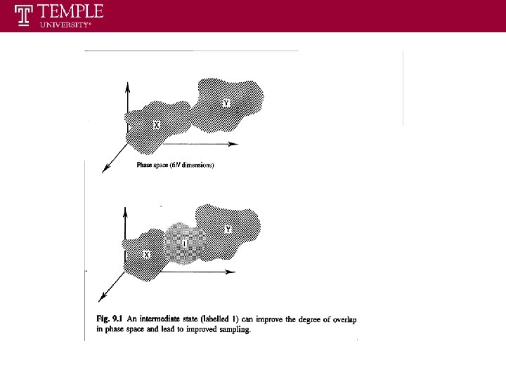
Intermediate States We can obviously extend this treatment to include multiple intermediate states with increasing overlap 0 1

Thermodynamic cycle to calculate binding free energy with restraint Protein (P) Ligand (L) Complex (PL) ΔF 0 Lelec+vdw ΔFwater PLelec+vdw ΔFprotein, restraint L PLrestraint+elec+vdw ΔFgas, restraint ΔFprotein ΔFgas= 0 Lrestraint PLrestraint

Relative binding free energy for two ligands Alchemical transformations - FEP

Relative binding free energy for two ligands Alchemical transformations - FEP Mutation of ligand A into ligand B in both the bound and the free states, following a different thermodynamic cycle. protein + ligand A ΔFAbinding protein ΔF 0 mutation protein + ligand B ligand ΔF 1 mutation ΔFBbinding protein ligand

Connection thermodynamics and kinetics O. Michielin, Ludwig Institute for Cancer Research, Epalinges,