Structural Analysis Lecture 8 Plane frame analysis using



- Slides: 52

Structural Analysis Lecture #8 Plane frame analysis using the stiffness method Dr. Wan Mohd Sabki Wan Omar Structure & Construction Engineering Email: wansabki@unimap. edu. my/ sabki. wanomar@griffithuni. edu. au Phone: 013 -9335477 1

Outline n n Frame-member stiffness matrix Displacement & Force transformation matrices Frame-member global stiffness matrix Application of the stiffness method for frame analysis 2

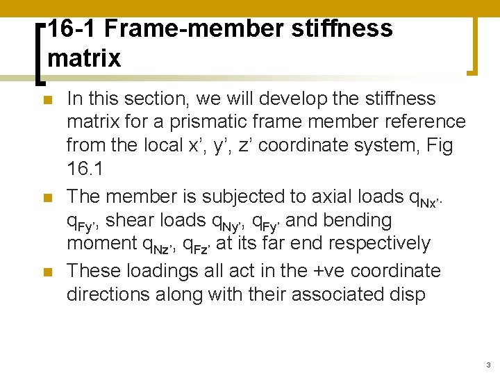
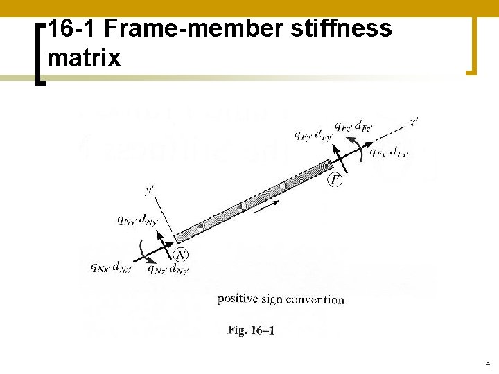
16 -1 Frame-member stiffness matrix n n n In this section, we will develop the stiffness matrix for a prismatic frame member reference from the local x’, y’, z’ coordinate system, Fig 16. 1 The member is subjected to axial loads q. Nx’. q. Fy’, shear loads q. Ny’, q. Fy’ and bending moment q. Nz’, q. Fz’ at its far end respectively These loadings all act in the +ve coordinate directions along with their associated disp 3

16 -1 Frame-member stiffness matrix 4

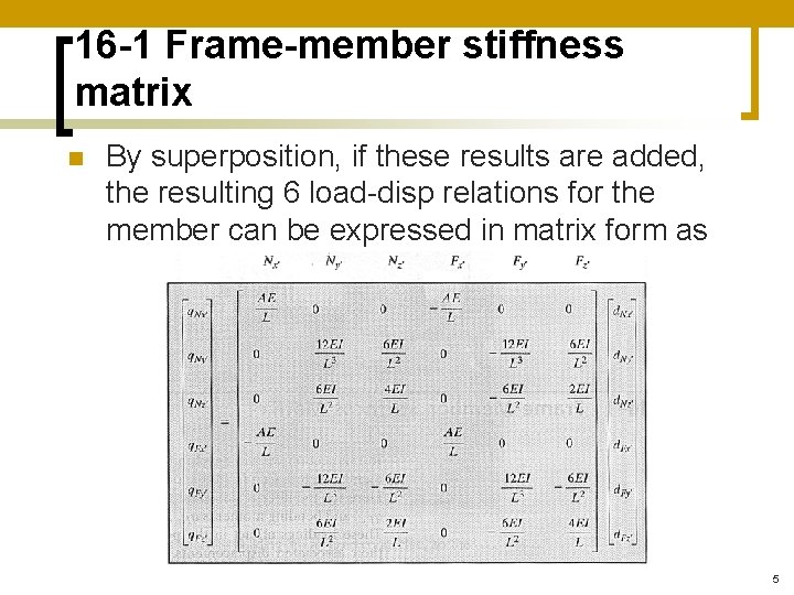
16 -1 Frame-member stiffness matrix n By superposition, if these results are added, the resulting 6 load-disp relations for the member can be expressed in matrix form as 5

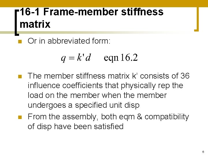
16 -1 Frame-member stiffness matrix n Or in abbreviated form: n The member stiffness matrix k’ consists of 36 influence coefficients that physically rep the load on the member when the member undergoes a specified unit disp From the assembly, both eqm & compatibility of disp have been satisfied n 6

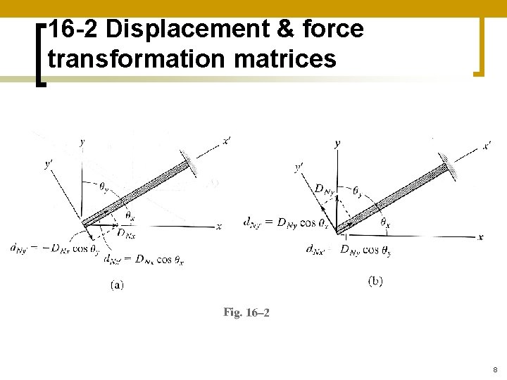
16 -2 Displacement & force transformation matrices n n We must be able to transform the internal member loads q & deformations d from local x’, y’, z’ coordinates to global x, y, z coordinates Disp transformation matrix ¡ Consider the frame member shown in Fig 16. 2(a) 7

16 -2 Displacement & force transformation matrices 8

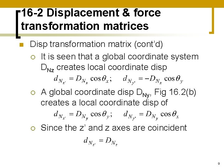
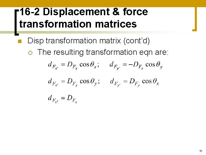
16 -2 Displacement & force transformation matrices n Disp transformation matrix (cont’d) ¡ It is seen that a global coordinate system DNz creates local coordinate disp ¡ A global coordinate disp DNy, Fig 16. 2(b) creates a local coordinate disp of ¡ Since the z’ and z axes are coincident 9

16 -2 Displacement & force transformation matrices n Disp transformation matrix (cont’d) ¡ The resulting transformation eqn are: 10

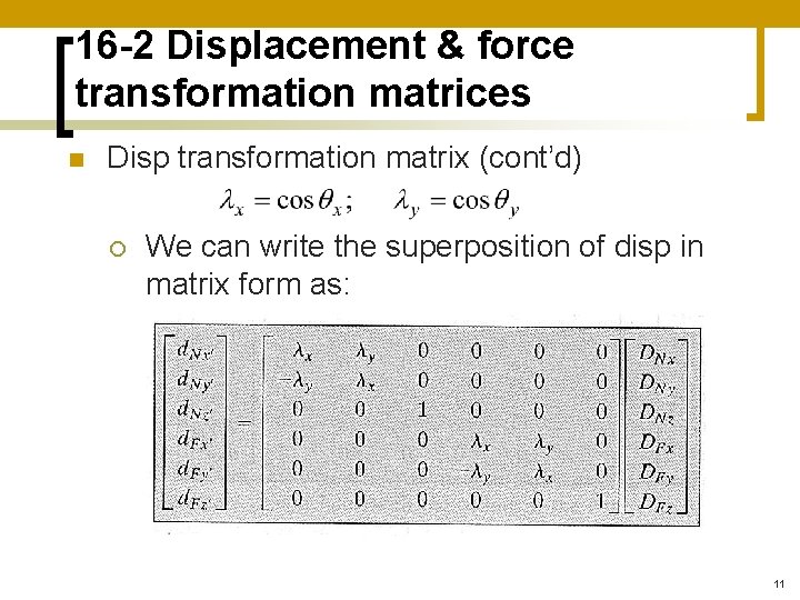
16 -2 Displacement & force transformation matrices n Disp transformation matrix (cont’d) ¡ We can write the superposition of disp in matrix form as: 11

16 -2 Displacement & force transformation matrices ¡ ¡ ¡ Or d = TD T transforms the 6 global x, y, z disp D into the 6 local x’, y’, z’ disp d T is referred to as the disp transformation matrix 12

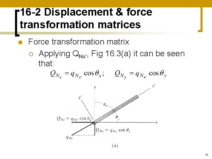
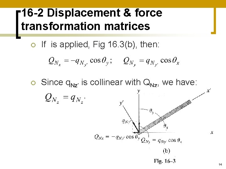
16 -2 Displacement & force transformation matrices n Force transformation matrix ¡ Applying QNx’, Fig 16. 3(a) it can be seen that: 13

16 -2 Displacement & force transformation matrices ¡ If is applied, Fig 16. 3(b), then: ¡ Since q. Nz’ is collinear with QNz, we have: 14

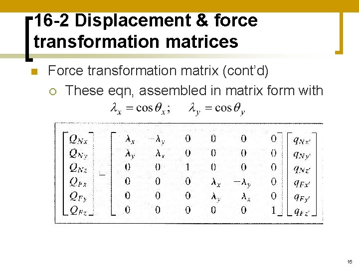
16 -2 Displacement & force transformation matrices n Force transformation matrix (cont’d) ¡ These eqn, assembled in matrix form with 15

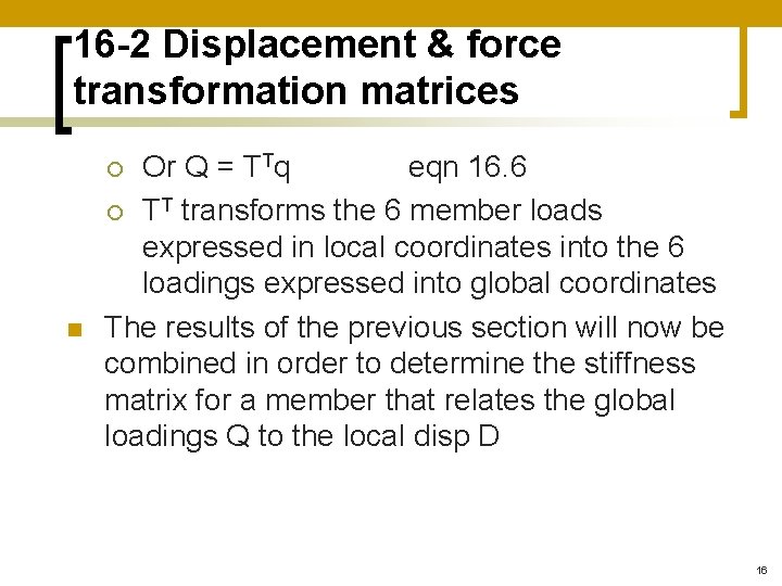
16 -2 Displacement & force transformation matrices Or Q = TTq eqn 16. 6 ¡ TT transforms the 6 member loads expressed in local coordinates into the 6 loadings expressed into global coordinates The results of the previous section will now be combined in order to determine the stiffness matrix for a member that relates the global loadings Q to the local disp D ¡ n 16

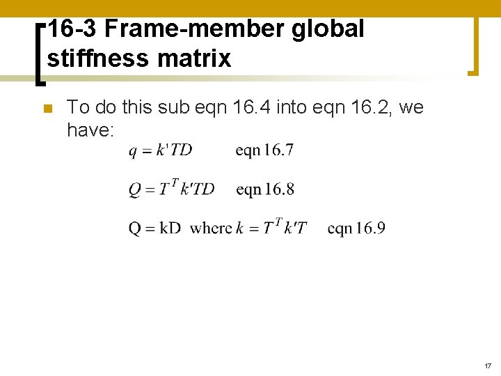
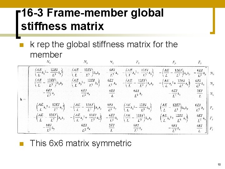
16 -3 Frame-member global stiffness matrix n To do this sub eqn 16. 4 into eqn 16. 2, we have: 17

16 -3 Frame-member global stiffness matrix n k rep the global stiffness matrix for the member n This 6 x 6 matrix symmetric 18

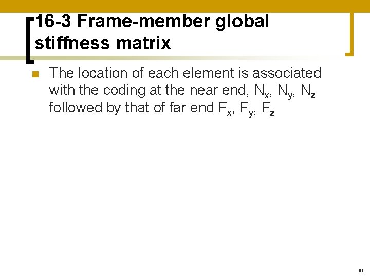
16 -3 Frame-member global stiffness matrix n The location of each element is associated with the coding at the near end, Nx, Ny, Nz followed by that of far end Fx, Fy, Fz 19

16 -4 Application of stiffness method for frame analysis n n Once the member stiffness matrices are established, they may be assembled into the structure stiffness matrix in the usual manner Lateral loads acting on a member, fabrication errors, temp changes, inclined supports & internal supports are handled in the same manner as was outlined for trusses & beams 20

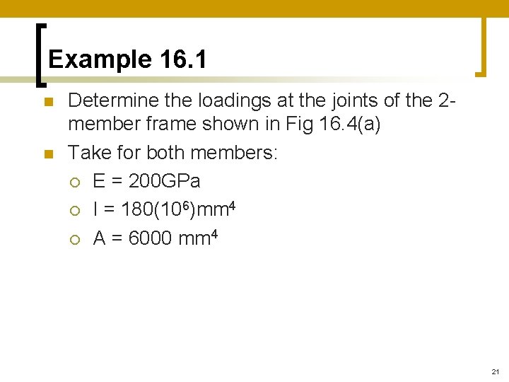
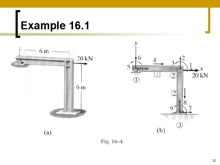
Example 16. 1 n n Determine the loadings at the joints of the 2 member frame shown in Fig 16. 4(a) Take for both members: ¡ E = 200 GPa ¡ I = 180(106)mm 4 ¡ A = 6000 mm 4 21

Example 16. 1 22

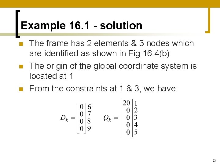
Example 16. 1 - solution n The frame has 2 elements & 3 nodes which are identified as shown in Fig 16. 4(b) The origin of the global coordinate system is located at 1 From the constraints at 1 & 3, we have: 23

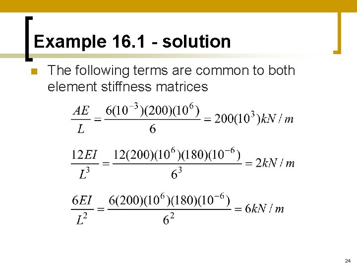
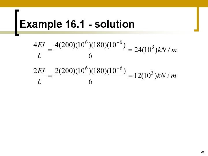
Example 16. 1 - solution n The following terms are common to both element stiffness matrices 24

Example 16. 1 - solution 25

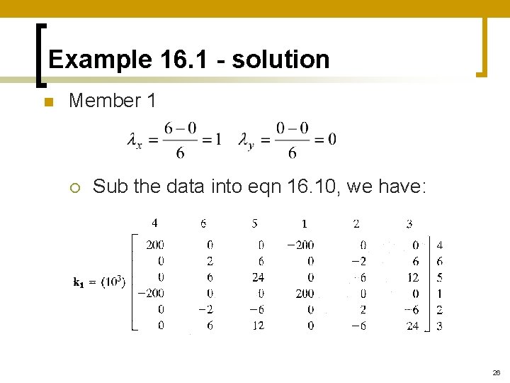
Example 16. 1 - solution n Member 1 ¡ Sub the data into eqn 16. 10, we have: 26

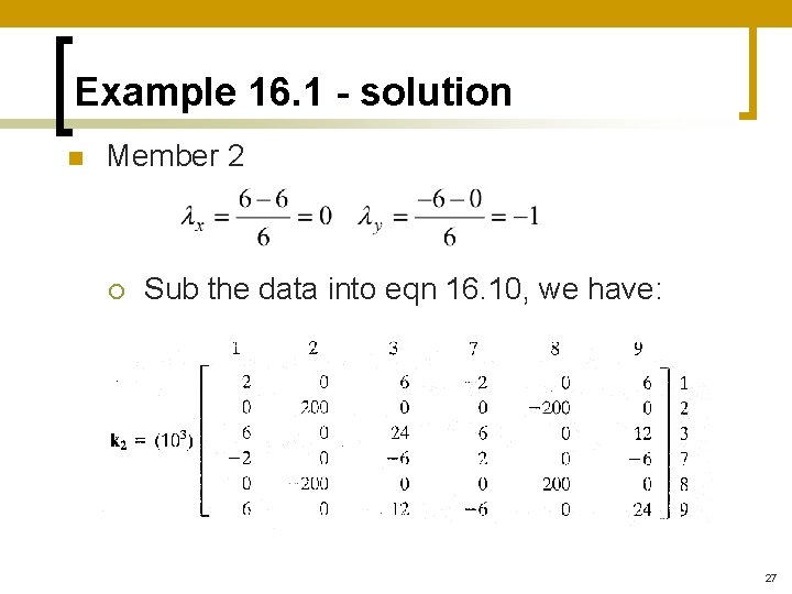
Example 16. 1 - solution n Member 2 ¡ Sub the data into eqn 16. 10, we have: 27

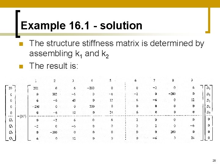
Example 16. 1 - solution n n The structure stiffness matrix is determined by assembling k 1 and k 2 The result is: 28

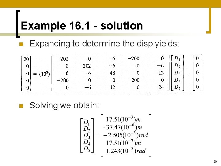
Example 16. 1 - solution n Expanding to determine the disp yields: n Solving we obtain: 29

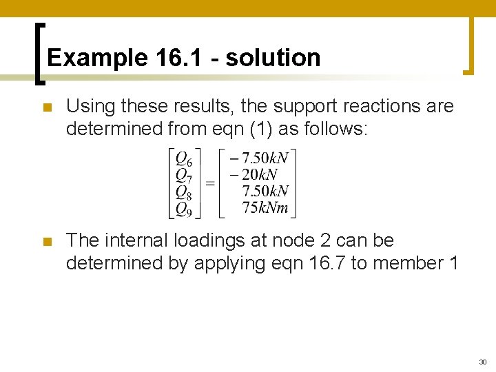
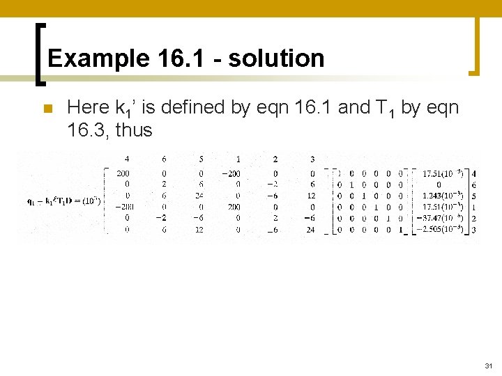
Example 16. 1 - solution n Using these results, the support reactions are determined from eqn (1) as follows: n The internal loadings at node 2 can be determined by applying eqn 16. 7 to member 1 30

Example 16. 1 - solution n Here k 1’ is defined by eqn 16. 1 and T 1 by eqn 16. 3, thus 31

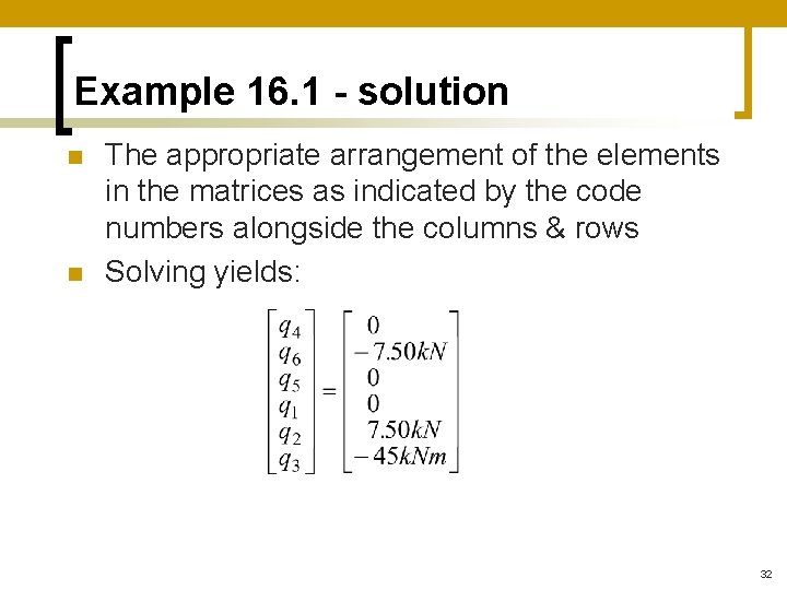
Example 16. 1 - solution n n The appropriate arrangement of the elements in the matrices as indicated by the code numbers alongside the columns & rows Solving yields: 32

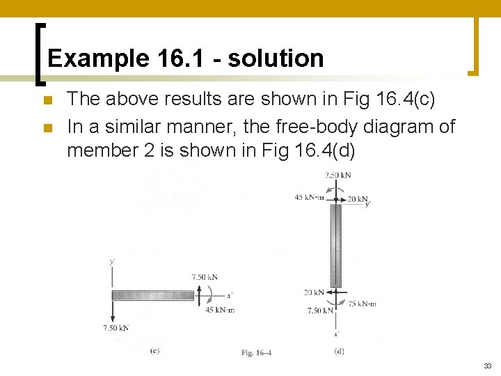
Example 16. 1 - solution n n The above results are shown in Fig 16. 4(c) In a similar manner, the free-body diagram of member 2 is shown in Fig 16. 4(d) 33

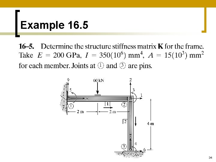
Example 16. 5 34

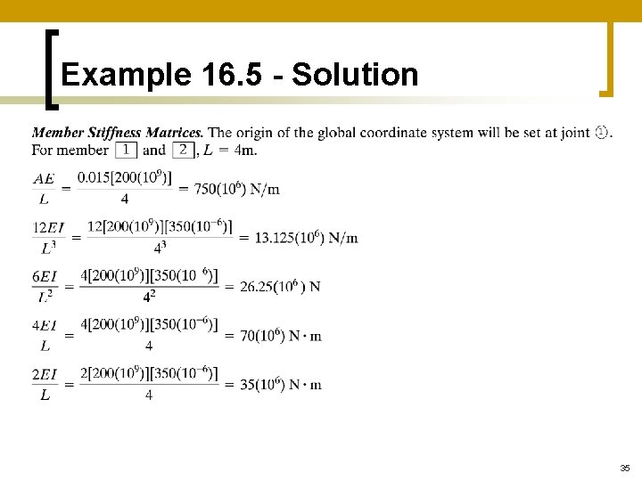
Example 16. 5 - Solution 35

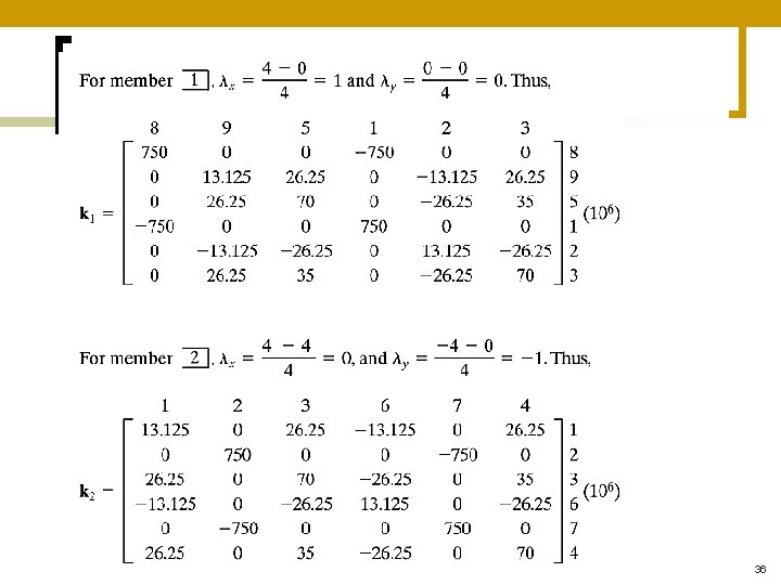
36

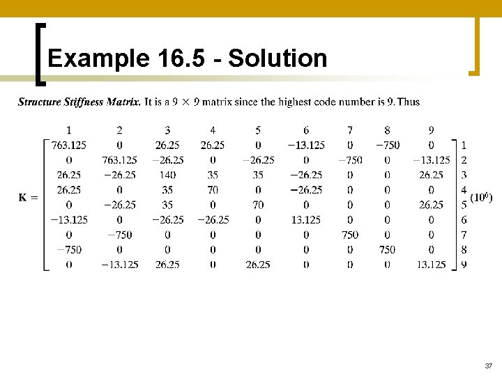
Example 16. 5 - Solution 37

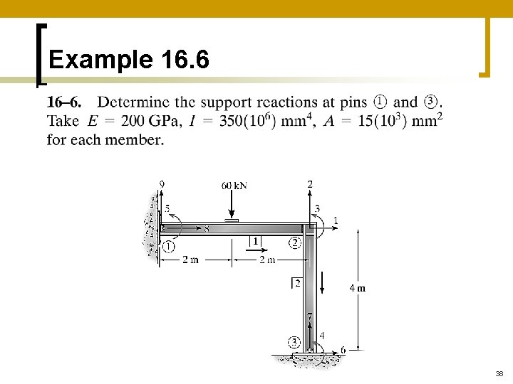
Example 16. 6 38

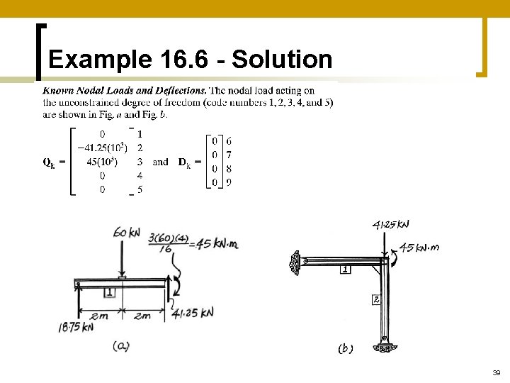
Example 16. 6 - Solution 39

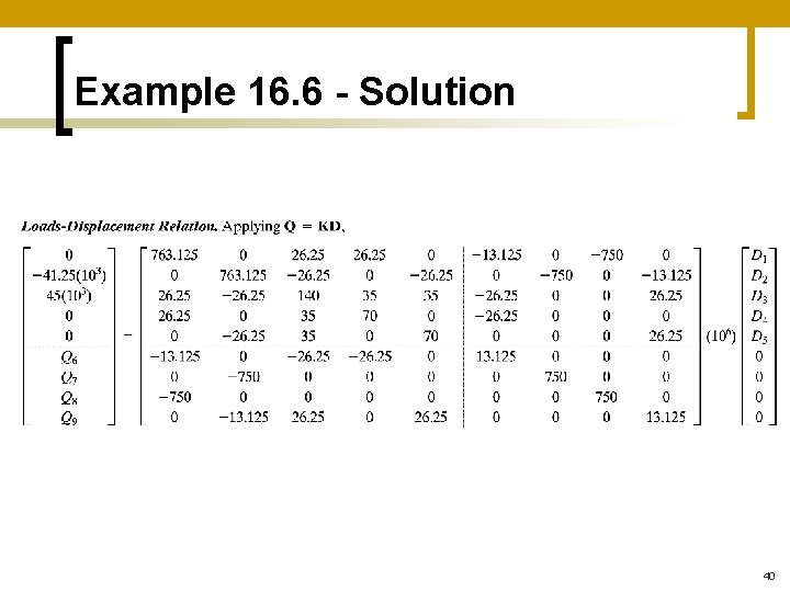
Example 16. 6 - Solution 40

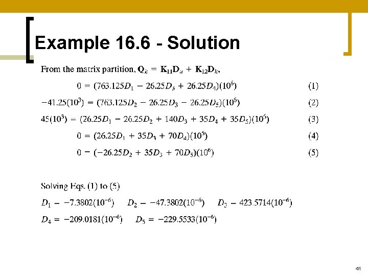
Example 16. 6 - Solution 41

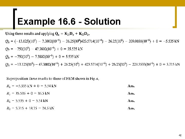
Example 16. 6 - Solution 42

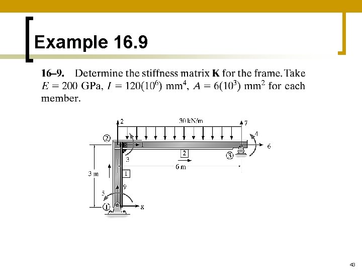
Example 16. 9 43

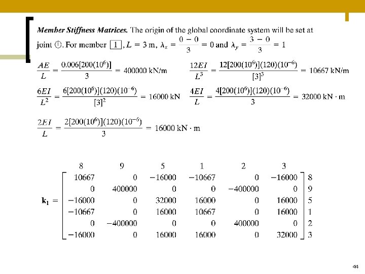
44

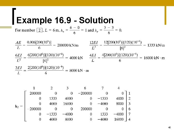
Example 16. 9 - Solution 45

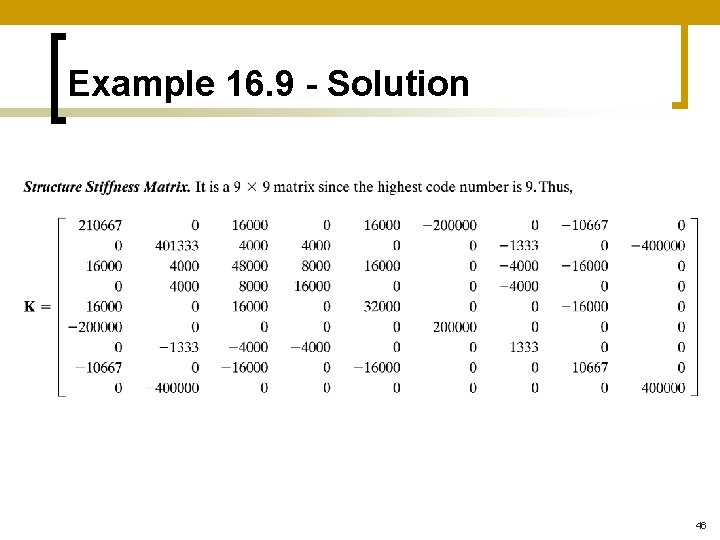
Example 16. 9 - Solution 46

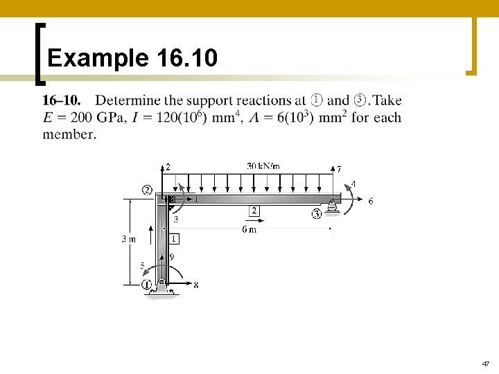
Example 16. 10 47

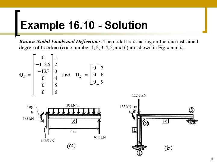
Example 16. 10 - Solution 48

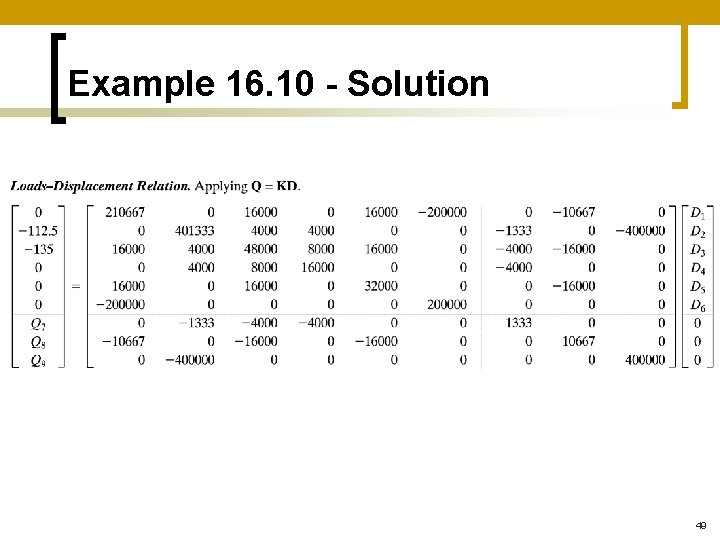
Example 16. 10 - Solution 49

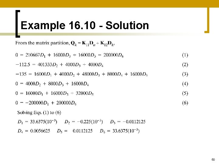
Example 16. 10 - Solution 50

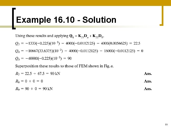
Example 16. 10 - Solution 51

52