Strong LP Formulations PrimalDual Approximation Algorithms David Shmoys

Strong LP Formulations & Primal-Dual Approximation Algorithms David Shmoys (joint work Tim Carnes & Maurice Cheung) June 23, 2011

Introduction n The standard approach to solve combinatorial integer programs in practice – start with a “simple” formulation & add valid inequalities Our agenda: show that same approach can be theoretically justified by approximation algorithms An ®-approximation algorithm produces a solution of cost within a factor of ® of the optimal solution in polynomial time

Introduction n Primal-dual method a leading approach in the design of approximation algorithms for NP-hard problems Consider several capacitated covering problems - covering knapsack problem - single-machine scheduling problems Give constant approximation algorithms based on strong linear programming (LP) formulations

Approximation Algorithms and LP n n n Use LP to design approximation algorithms Optimal value for LP gives bound on optimal integer programming (IP) value Want to find feasible IP solution of value within a factor of ® of optimal LP solution Key is to start with “right” LP relaxation LP-based approximation algorithm produces additional performance guarantee on each problem instance Empirical success of IP cutting plane methods suggests stronger formulations - needs theory!

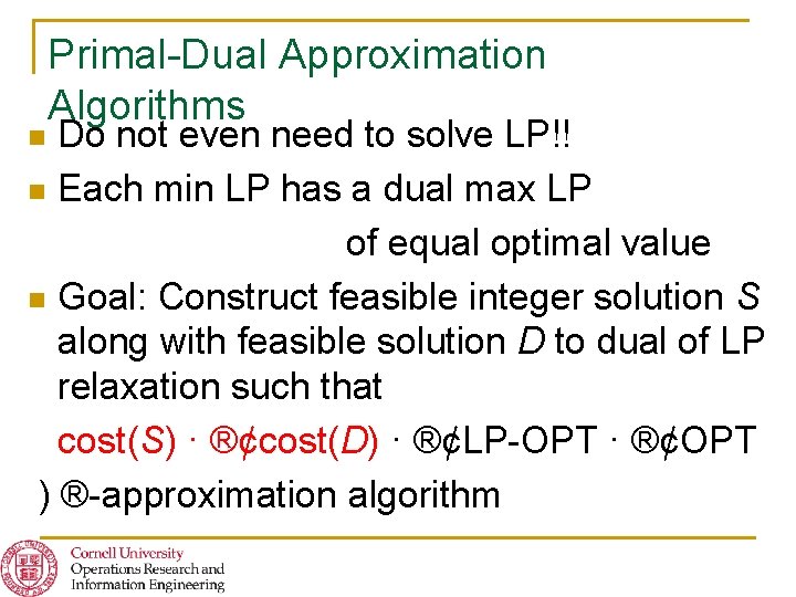
Primal-Dual Approximation Algorithms Do not even need to solve LP!! n Each min LP has a dual max LP of equal optimal value n Goal: Construct feasible integer solution S along with feasible solution D to dual of LP relaxation such that cost(S) · ®¢cost(D) · ®¢LP-OPT · ®¢OPT ) ®-approximation algorithm n

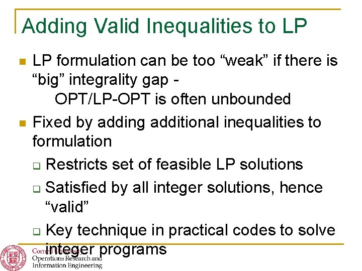
Adding Valid Inequalities to LP n n LP formulation can be too “weak” if there is “big” integrality gap OPT/LP-OPT is often unbounded Fixed by adding additional inequalities to formulation q Restricts set of feasible LP solutions q Satisfied by all integer solutions, hence “valid” q Key technique in practical codes to solve integer programs

Knapsack-Cover Inequalities n Carr, Fleischer, Leung and Phillips (2000) developed valid knapsack-cover inequalities and LP-rounding algorithms for several capacitated covering problems q Requires solving LP with ellipsoid method q Further complicated since inequalities are not known to be separable q GOAL: develop a primal-dual analog!

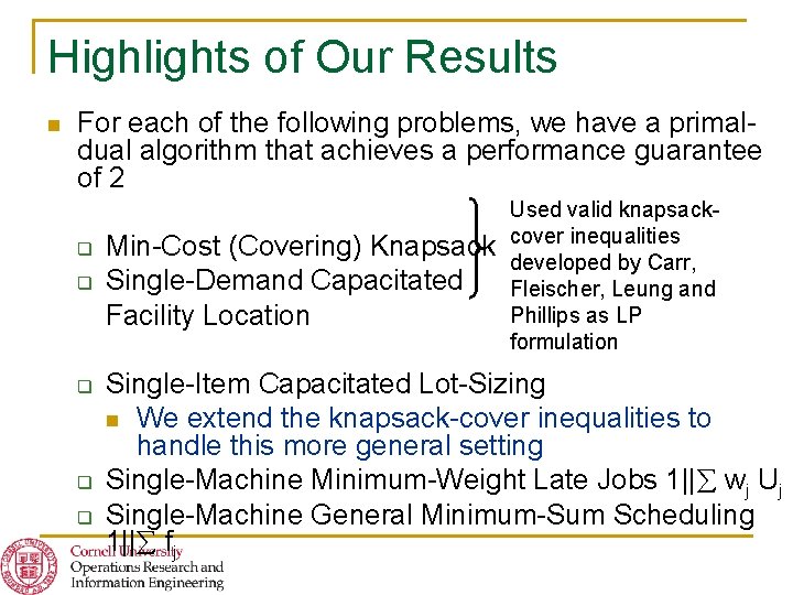
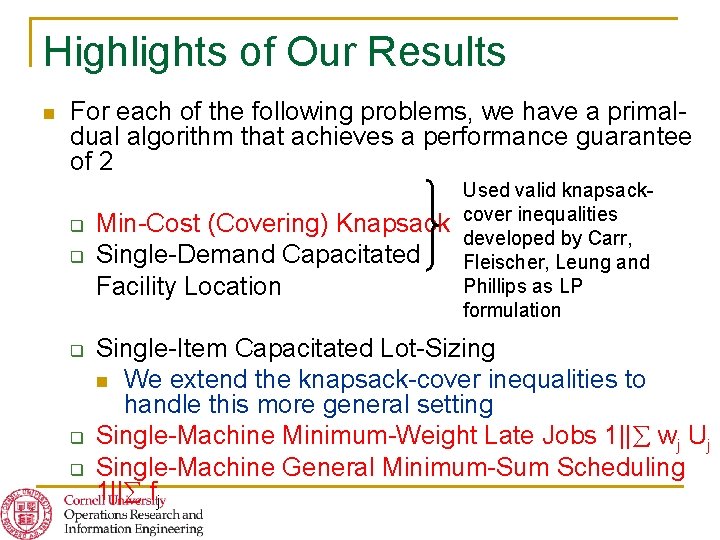
Highlights of Our Results n For each of the following problems, we have a primaldual algorithm that achieves a performance guarantee of 2 q q q Min-Cost (Covering) Knapsack Single-Demand Capacitated Facility Location Used valid knapsackcover inequalities developed by Carr, Fleischer, Leung and Phillips as LP formulation Single-Item Capacitated Lot-Sizing n We extend the knapsack-cover inequalities to handle this more general setting Single-Machine Minimum-Weight Late Jobs 1|| wj Uj Single-Machine General Minimum-Sum Scheduling 1|| fj

Highlights of Our Results n For each of the following problems, we have a primaldual algorithm that achieves a performance guarantee of 2 q q q Min-Cost (Covering) Knapsack Single-Demand Capacitated Facility Location Used valid knapsackcover inequalities developed by Carr, Fleischer, Leung and Phillips as LP formulation Single-Item Capacitated Lot-Sizing n We extend the knapsack-cover inequalities to handle this more general setting Single-Machine Minimum-Weight Late Jobs 1|| wj Uj Single-Machine General Minimum-Sum Scheduling 1|| fj

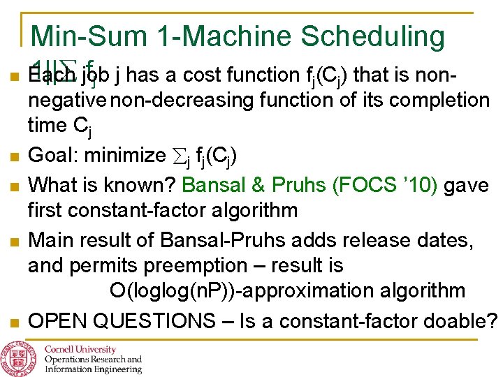
Min-Sum 1 -Machine Scheduling n n n 1|| job fj j has a cost function fj(Cj) that is non. Each negative non-decreasing function of its completion time Cj Goal: minimize j fj(Cj) What is known? Bansal & Pruhs (FOCS ’ 10) gave first constant-factor algorithm Main result of Bansal-Pruhs adds release dates, and permits preemption – result is O(loglog(n. P))-approximation algorithm OPEN QUESTIONS – Is a constant-factor doable?

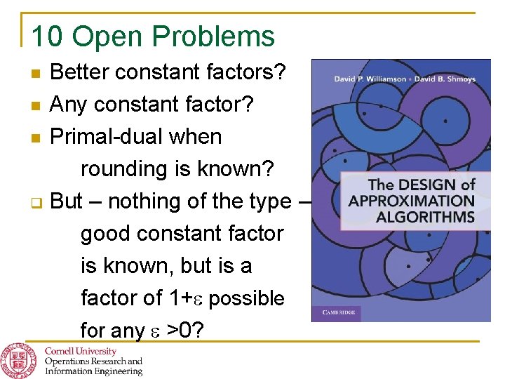
10 Open Problems Better constant factors? n Any constant factor? n Primal-dual when rounding is known? q But – nothing of the type – good constant factor is known, but is a factor of 1+ possible for any >0? n

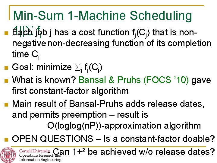
Min-Sum 1 -Machine Scheduling n n n 1|| job fj j has a cost function fj(Cj) that is non. Each negative non-decreasing function of its completion time Cj Goal: minimize j fj(Cj) What is known? Bansal & Pruhs (FOCS ’ 10) gave first constant-factor algorithm Main result of Bansal-Pruhs adds release dates, and permits preemption – result is O(loglog(n. P))-approximation algorithm OPEN QUESTIONS – Is a constant-factor doable? - Can 1+² be achieved w/o release dates?

Primal-Dual for Covering Problems n n Early primal-dual algorithms q Bar-Yehuda and Even (1981) – weighted vertex cover q Chvátal (1979) – weighted set cover Agrawal, Klein and Ravi (1995) Goemans and Williamson (1995) generalized Steiner (cut covering) problems Bertismas & Teo (1998) Jain & Vazirani (1999) uncapacitated facility location problem Inventory problems q Levi, Roundy and Shmoys (2006)

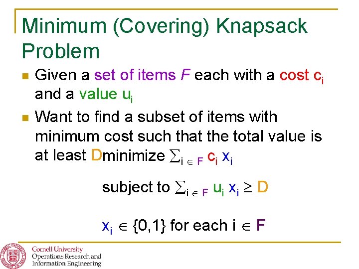
Minimum (Covering) Knapsack Problem n n Given a set of items F each with a cost ci and a value ui Want to find a subset of items with minimum cost such that the total value is at least Dminimize i F ci xi subject to i F ui xi D xi {0, 1} for each i F

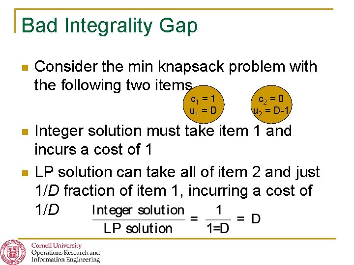
Bad Integrality Gap n Consider the min knapsack problem with the following two items c 1 = 1 u 1 = D n n c 2 = 0 u 2 = D-1 Integer solution must take item 1 and incurs a cost of 1 LP solution can take all of item 2 and just 1/D fraction of item 1, incurring a cost of 1/D

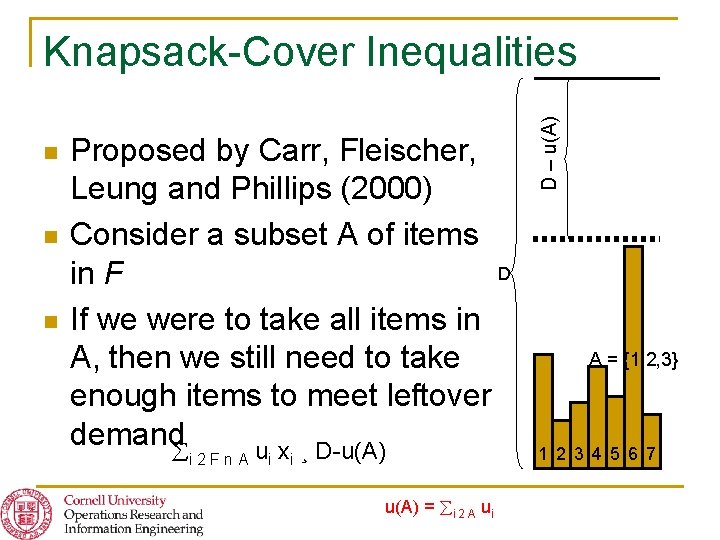
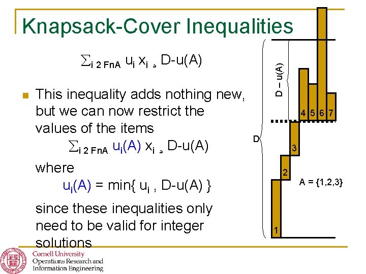
n n n Proposed by Carr, Fleischer, Leung and Phillips (2000) Consider a subset A of items D in F If we were to take all items in A, then we still need to take enough items to meet leftover demand u x ¸ D-u(A) i 2 Fn. A i i u(A) = i 2 A ui D – u(A) Knapsack-Cover Inequalities A = {1, 2, 3} 1 2 3 4 5 6 7

Knapsack-Cover Inequalities n This inequality adds nothing new, but we can now restrict the values of the items i 2 Fn. A ui(A) xi ¸ D-u(A) D – u(A) i 2 Fn. A ui xi ¸ D-u(A) 4 5 6 7 D 3 where ui(A) = min{ ui , D-u(A) } since these inequalities only need to be valid for integer solutions 2 1 A = {1, 2, 3}

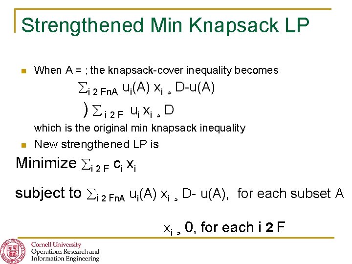
Strengthened Min Knapsack LP n When A = ; the knapsack-cover inequality becomes i 2 Fn. A ui(A) xi ¸ D-u(A) ) i 2 F ui x i ¸ D which is the original min knapsack inequality n New strengthened LP is Minimize i 2 F ci xi subject to i 2 Fn. A ui(A) xi ¸ D- u(A), for each subset A xi ¸ 0, for each i 2 F

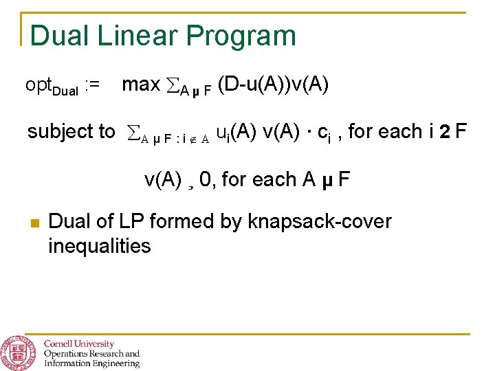
Dual Linear Program opt. Dual : = max A µ F (D-u(A))v(A) subject to A µ F : i A ui(A) v(A) · ci , for each i 2 F v(A) ¸ 0, for each A µ F n Dual of LP formed by knapsack-cover inequalities

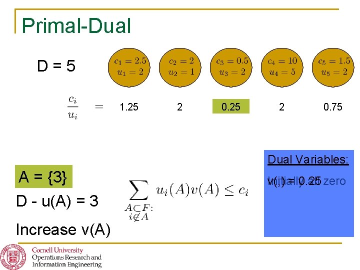
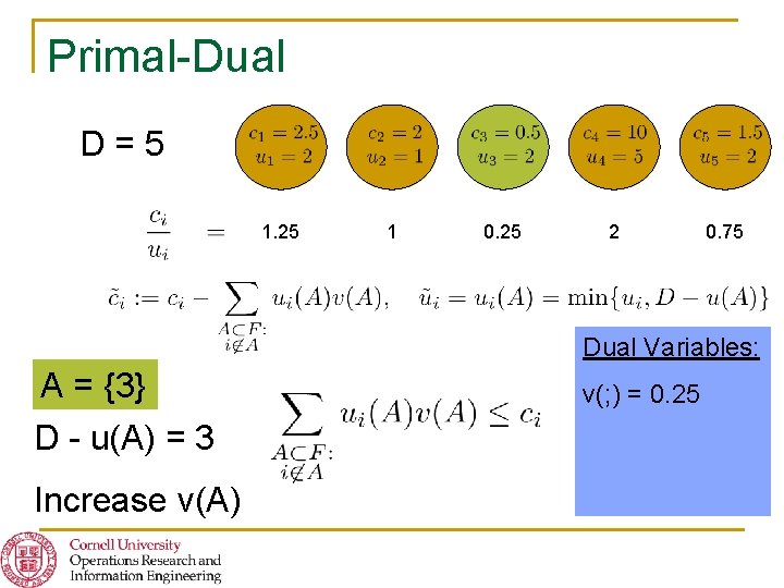
Primal-Dual D=5 1. 25 2 0. 75 Dual Variables: A = {3} ; D - u(A) = 3 5 Increase v(A) Initially v(; ) = 0. 25 all zero

Primal-Dual D=5 1. 25 1 0. 25 2 0. 75 Dual Variables: A = {3} D - u(A) = 3 Increase v(A) v(; ) = 0. 25

Primal-Dual D=5 1. 25 1 0. 25 2 0. 75 Dual Variables: A = {3} D - u(A) = 3 Increase v(A) v(; ) = 0. 25

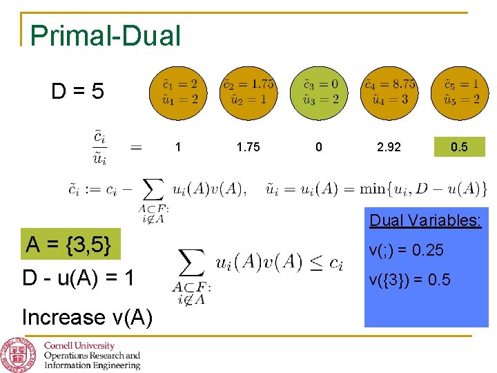
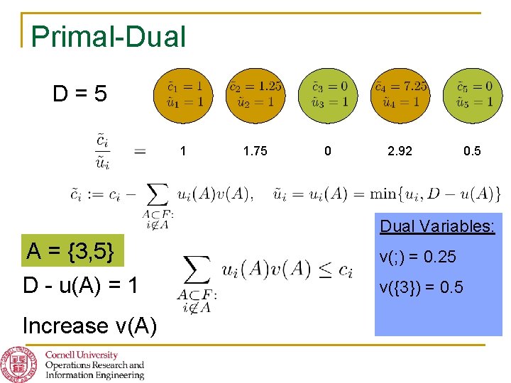
Primal-Dual D=5 1 1. 75 0 2. 92 0. 5 Dual Variables: A = {3, 5} {3} D - u(A) = 1 3 Increase v(A) v(; ) = 0. 25 v({3}) = 0. 5

Primal-Dual D=5 1 1. 75 0 2. 92 0. 5 Dual Variables: A = {3, 5} {3} D - u(A) = 1 Increase v(A) v(; ) = 0. 25 v({3}) = 0. 5

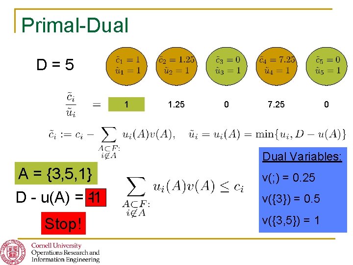
Primal-Dual D=5 1 1. 25 0 7. 25 0 Dual Variables: A = {3, 5, 1} {3, 5} {3} D - u(A) = -1 1 Stop!v(A) Increase v(; ) = 0. 25 v({3}) = 0. 5 v({3, 5}) = 1

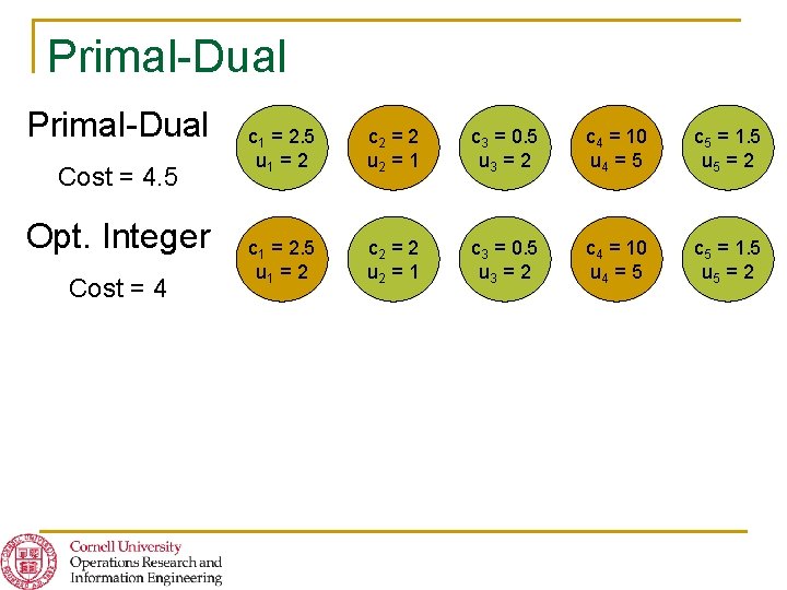
Primal-Dual Cost = 4. 5 Opt. Integer Cost = 4 c 1 = 2. 5 u 1 = 2 c 2 = 2 u 2 = 1 c 3 = 0. 5 u 3 = 2 c 4 = 10 u 4 = 5 c 5 = 1. 5 u 5 = 2

Primal-Dual Summary n n n Start with all variables set to zero and solution A as the empty set Increase variable v(A) until a dual constraint becomes tight for some item i Add item i to solution A and repeat Stop once solution A has large enough value to meet demand D Call final solution S and set xi = 1 for all i 2 S

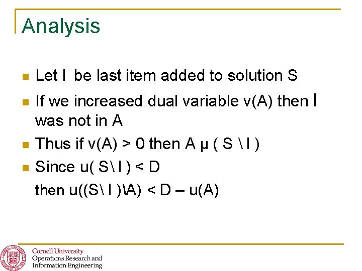
Analysis n n Let l be last item added to solution S If we increased dual variable v(A) then l was not in A Thus if v(A) > 0 then A µ ( S l ) Since u( S l ) < D then u((S l )A) < D – u(A)

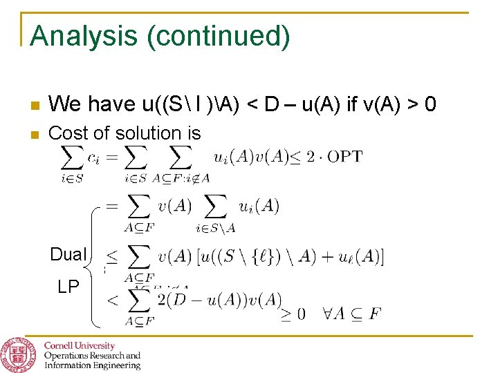
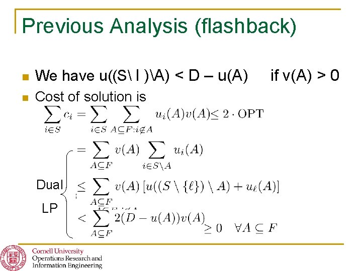
Analysis (continued) n We have u((S l )A) < D – u(A) if v(A) > 0 n Cost of solution is Dual LP

Primal-Dual Theorem For the min-cost covering knapsack problem, the LP relaxation with knapsackcover inequalities can be used to derive a (simple) primal-dual 2 -approximation algorithm.

Knapsack-Cover Inequalities Everywhere n n n Bansal, Buchbinder, Naor (2008) Randomized competitive algorithms for generalized caching (and weighted paging) Bansal, Gupta, & Krishnaswamy (2010) 485 approximation algorithm for min-sum set cover Bansal & Pruhs (2010) O(log n. P)-approximation algorithm for general 1 -machine preemptive scheduling + O(1) with identical deadlines

Minimum-Weight Late Jobs on 1 Machine n n Each job j has processing time pj , deadline dj, weight wj Choose a subset L of jobs of minimum-weight to be late - not scheduled to complete by deadline This problem is (weakly) NP-hard can be solved in O( n j pj ) time [Lawler & Moore], (1+²)-approximation in O(n 3/²) time [Sahni] If there also are release dates that constrain when a job may start, no approximation result is possible - focus on max-weight set of jobs scheduled on time [Bar. Noy, Bar-Yehuda, Freund, Naor, & Schieber] allow preemption [Bansal & Pruhs]

What if all deadlines are the same? n n n Total processing time is j pj ! P WLOG assume schedule runs through [0, P] Deadline D ) at least P-D units of processing are done after D So just select set of total processing at least P-D of minimum total weight , minimum-cost covering knapsack problem

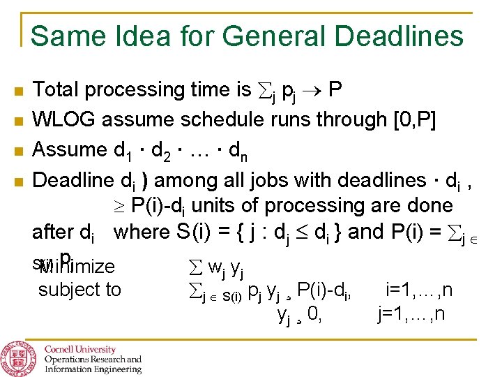
Same Idea for General Deadlines n n Total processing time is j pj P WLOG assume schedule runs through [0, P] Assume d 1 · d 2 · … · dn Deadline di ) among all jobs with deadlines · di , P(i)-di units of processing are done after di where S(i) = { j : dj di } and P(i) = j pj S(i) Minimize w y subject to j j j S(i) pj yj ¸ P(i)-di, yj ¸ 0, i=1, …, n j=1, …, n

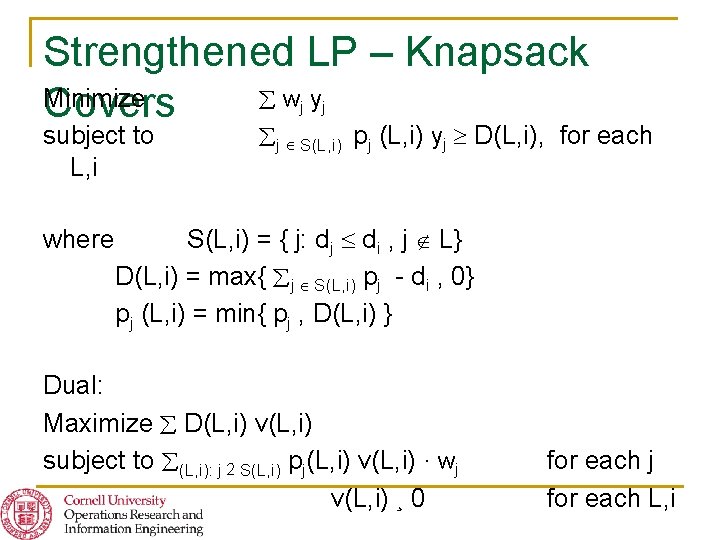
Strengthened LP – Knapsack Minimize w y Covers j subject to L, i where j j S(L, i) pj (L, i) yj D(L, i), for each S(L, i) = { j: dj di , j L} D(L, i) = max{ j S(L, i) pj - di , 0} pj (L, i) = min{ pj , D(L, i) } Dual: Maximize D(L, i) v(L, i) subject to (L, i): j 2 S(L, i) pj(L, i) v(L, i) · wj v(L, i) ¸ 0 for each j for each L, i

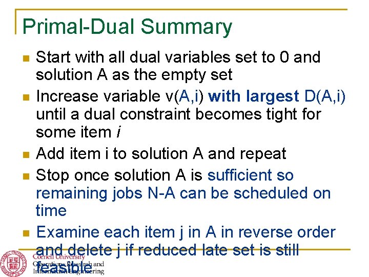
Primal-Dual Summary n n n Start with all dual variables set to 0 and solution A as the empty set Increase variable v(A, i) with largest D(A, i) until a dual constraint becomes tight for some item i Add item i to solution A and repeat Stop once solution A is sufficient so remaining jobs N-A can be scheduled on time Examine each item j in A in reverse order and delete j if reduced late set is still feasible

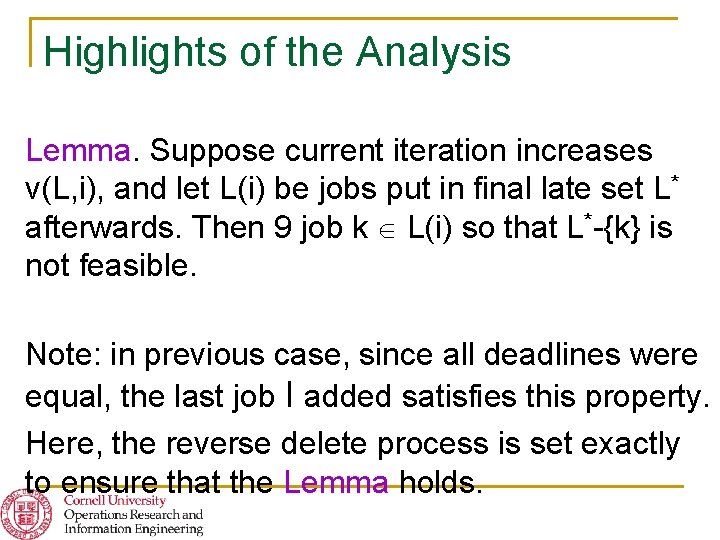
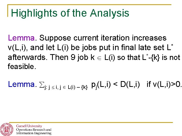
Highlights of the Analysis Lemma. Suppose current iteration increases v(L, i), and let L(i) be jobs put in final late set L* afterwards. Then 9 job k L(i) so that L*-{k} is not feasible. Note: in previous case, since all deadlines were equal, the last job l added satisfies this property. Here, the reverse delete process is set exactly to ensure that the Lemma holds.

Highlights of the Analysis Lemma. Suppose current iteration increases v(L, i), and let L(i) be jobs put in final late set L* afterwards. Then 9 job k L(i) so that L*-{k} is not feasible. Lemma. j: j i, j L(i) – {k} pj(L, i) < D(L, i) if v(L, i)>0.

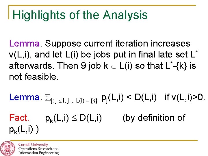
Highlights of the Analysis Lemma. Suppose current iteration increases v(L, i), and let L(i) be jobs put in final late set L* afterwards. Then 9 job k L(i) so that L*-{k} is not feasible. Lemma. j: j i, j L(i) – {k} pj(L, i) < D(L, i) if v(L, i)>0. Fact. pk(L, i) D(L, i) pk(L, i) ) (by definition of

Highlights of the Analysis Lemma. Suppose current iteration increases v(L, i), and let L(i) be jobs put in final late set L* afterwards. Then 9 job k L(i) so that L*-{k} is not feasible. Lemma. j: j i, j L(i) – {k} pj(L, i) < D(L, i) if v(L, i)>0. Fact. pk(L, i) D(L, i) pk(L, i) ) (by definition of

Previous Analysis (flashback) n We have u((S l )A) < D – u(A) n Cost of solution is Dual LP if v(A) > 0

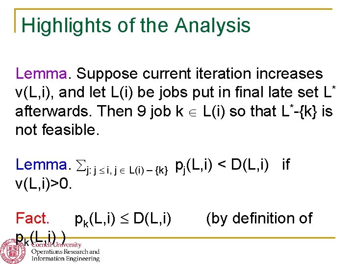
Highlights of the Analysis Lemma. Suppose current iteration increases v(L, i), and let L(i) be jobs put in final late set L* afterwards. Then 9 job k L(i) so that L*-{k} is not feasible. Lemma. j: j i, j L(i) – {k} pj(L, i) < D(L, i) if v(L, i)>0. Fact. pk(L, i) D(L, i) pk(L, i) ) (by definition of

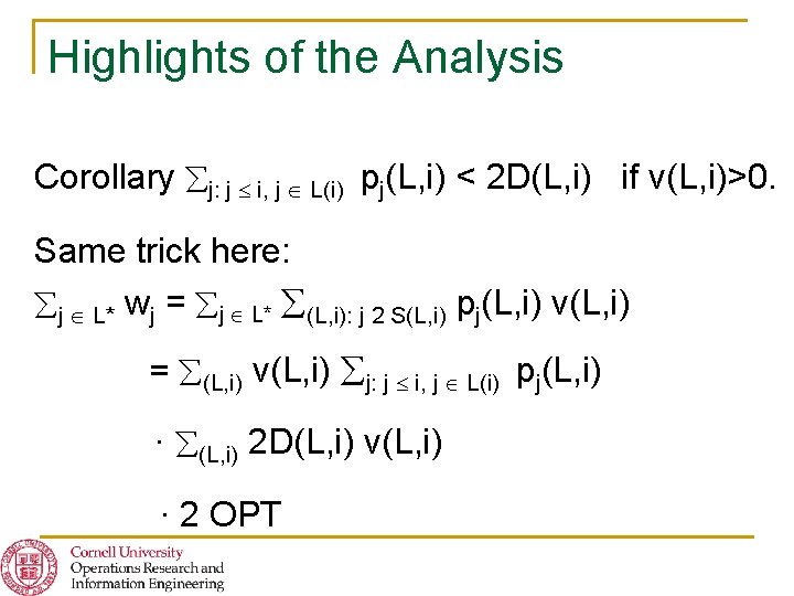
Highlights of the Analysis Corollary j: j i, j L(i) pj(L, i) < 2 D(L, i) if v(L, i)>0. Same trick here: j L* wj = j L* (L, i): j 2 S(L, i) pj(L, i) v(L, i) = (L, i) v(L, i) j: j i, j L(i) pj(L, i) · (L, i) 2 D(L, i) v(L, i) · 2 OPT

Primal-Dual Theorem For the 1 -machine min-weight late jobs scheduling problem with a common deadline, the LP relaxation with knapsackcover inequalities can be used to derive a (simple) primal-dual 2 -approximation algorithm.

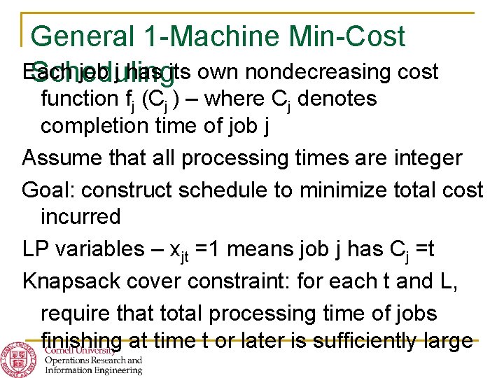
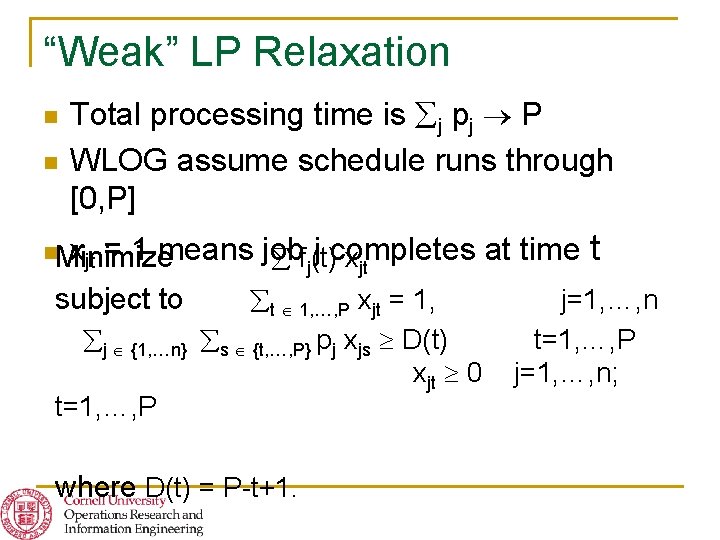
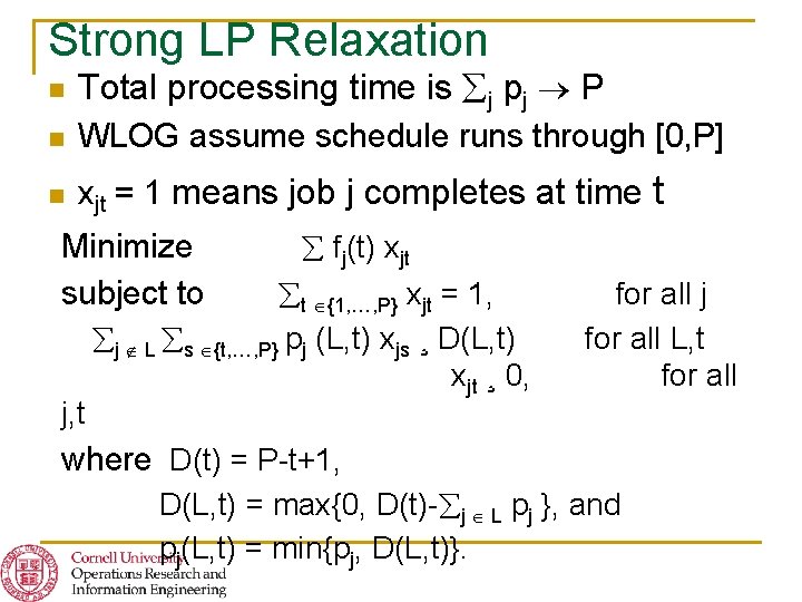
General 1 -Machine Min-Cost Each job j has its own nondecreasing cost Scheduling function fj (Cj ) – where Cj denotes completion time of job j Assume that all processing times are integer Goal: construct schedule to minimize total cost incurred LP variables – xjt =1 means job j has Cj =t Knapsack cover constraint: for each t and L, require that total processing time of jobs finishing at time t or later is sufficiently large

Primal-Dual Theorem(s) For 1 -machine min-cost scheduling, LP relaxation with knapsack-cover inequalities can be used to derive a (simple) primal-dual pseudo-polynomial 2 -approximation algorithm. For 1 -machine min-cost scheduling, LP relaxation with knapsack-cover inequalities can be used to derive a (simple) primal-dual (2+²)-approximation algorithm.

“Weak” LP Relaxation n n Total processing time is j pj P WLOG assume schedule runs through [0, P] = 1 means job j completes at time t fj(t) xjt n. Minimize xjt subject to j {1, …n} t=1, …, P t 1, …, P xjt = 1, s {t, …, P} pj xjs D(t) xjt 0 where D(t) = P-t+1. j=1, …, n t=1, …, P j=1, …, n;

Strong LP Relaxation n Total processing time is j pj P n WLOG assume schedule runs through [0, P] n xjt = 1 means job j completes at time fj(t) xjt t {1, …, P} xjt = 1, j L s {t, …, P} pj (L, t) xjs ¸ D(L, t) xjt ¸ 0, Minimize subject to j, t t for all j for all L, t for all where D(t) = P-t+1, D(L, t) = max{0, D(t)- j L pj }, and pj(L, t) = min{pj, D(L, t)}.

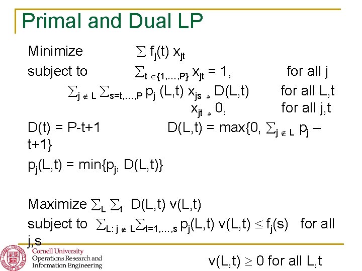
Primal and Dual LP Minimize fj(t) xjt subject to t {1, …, P} xjt = 1, for all j j L s=t, …, P pj (L, t) xjs ¸ D(L, t) for all L, t xjt ¸ 0, for all j, t D(t) = P-t+1 D(L, t) = max{0, j L pj – t+1} pj(L, t) = min{pj, D(L, t)} Maximize L t D(L, t) v(L, t) subject to L: j L t=1, …, s pj(L, t) v(L, t) fj(s) for all j, s v(L, t) 0 for all L, t

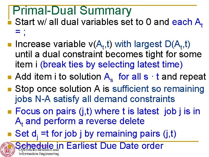
Primal-Dual Summary n n n n Start w/ all dual variables set to 0 and each At =; Increase variable v(At, t) with largest D(At, t) until a dual constraint becomes tight for some item i (break ties by selecting latest time) Add item i to solution As for all s · t and repeat Stop once solution A is sufficient so remaining jobs N-A satisfy all demand constraints Focus on pairs (j, t) where t is latest job j is in At and perform a reverse delete Set dj =t for job j by remaining pairs (j, t) Schedule in Earliest Due Date order

Primal-Dual Theorem For 1 -machine min-cost scheduling, LP relaxation with knapsack-cover inequalities can be used to derive a (simple) primal-dual pseudo-polynomial 2 -approximation algorithm.

Removing the “Pseudo” with a (1+²) § This requires only standard Loss techniques § For each job j, partition the potential job completion times {1, …, P} into blocks so that within block the cost for j increases by · 1+² § Consider finest partition based on all n jobs § Now consider variables xjt that assign job j to finish in block t of this partition. Fringe Benefit: more general models, § All other details remain basically the same. such as possible periods of machine non-availability

Primal-Dual Theorem For 1 -machine min-cost scheduling, LP relaxation with knapsack-cover inequalities can be used to derive a (simple) primal-dual (2+²)approximation algorithm.

Some Open Problems n n Give a constant approximation algorithm for 1 -machine min-sum scheduling with release dates allowing preemption Give a (1+²)-approximation algorithm for 1 machine min-sum scheduling, for arbitrarily small ² > 0 Give an LP-based constant approximation algorithm for capacitated facility location Use “configuration LP” to find an approximation algorithm for bin-packing problem that uses at most ONE bin more than optimal

Thank you! n Any questions?