StripPlot Designs Sometimes called splitblock design For experiments

Strip-Plot Designs ü Sometimes called split-block design ü For experiments involving factors that are difficult to apply to small plots ü Three sizes of plots so there are three experimental errors ü The interaction is measured with greater precision than the main effects

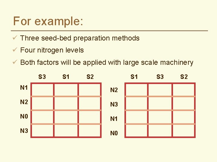
For example: ü Three seed-bed preparation methods ü Four nitrogen levels ü Both factors will be applied with large scale machinery S 3 S 1 S 2 S 1 N 2 N 3 N 0 N 1 N 3 N 0 S 3 S 2

Advantages --- Disadvantages ü Advantages – Permits efficient application of factors that would be difficult to apply to small plots ü Disadvantages – Differential precision in the estimation of interaction and the main effects – Complicated statistical analysis

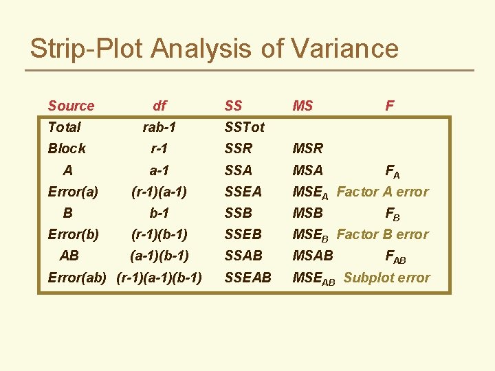
Strip-Plot Analysis of Variance Source df SS MS F Total rab-1 Block r-1 SSR MSR A a-1 SSA MSA SSEA MSEA Factor A error SSB MSB (r-1)(b-1) SSEB MSEB Factor B error (a-1)(b-1) SSAB MSAB SSEAB MSEAB Subplot error Error(a) B Error(b) AB (r-1)(a-1) b-1 Error(ab) (r-1)(a-1)(b-1) SSTot FA FB FAB

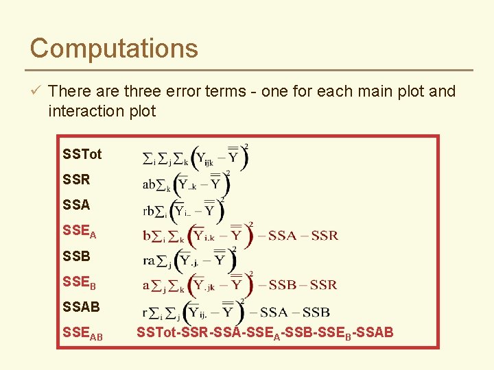
Computations ü There are three error terms - one for each main plot and interaction plot SSTot SSR SSA SSEA SSB SSEB SSAB SSEAB SSTot-SSR-SSA-SSEA-SSB-SSEB-SSAB

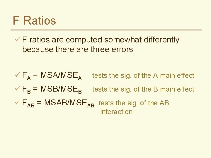
F Ratios ü F ratios are computed somewhat differently because there are three errors ü FA = MSA/MSEA tests the sig. of the A main effect ü FB = MSB/MSEB tests the sig. of the B main effect ü FAB = MSAB/MSEAB tests the sig. of the AB interaction

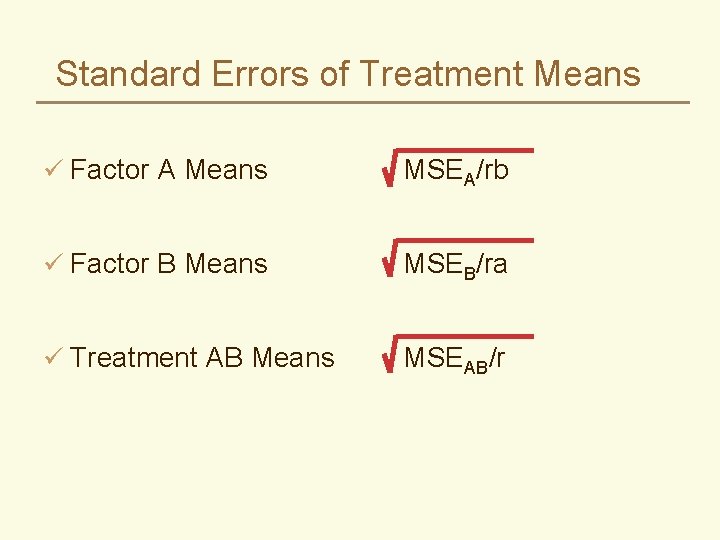
Standard Errors of Treatment Means ü Factor A Means MSEA/rb ü Factor B Means MSEB/ra ü Treatment AB Means MSEAB/r

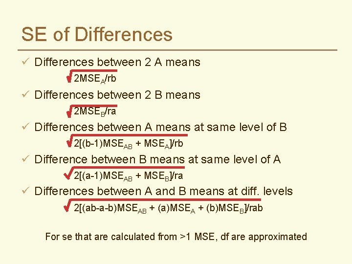
SE of Differences ü Differences between 2 A means 2 MSEA/rb ü Differences between 2 B means 2 MSEB/ra ü Differences between A means at same level of B 2[(b-1)MSEAB + MSEA]/rb ü Difference between B means at same level of A 2[(a-1)MSEAB + MSEB]/ra ü Differences between A and B means at diff. levels 2[(ab-a-b)MSEAB + (a)MSEA + (b)MSEB]/rab For se that are calculated from >1 MSE, df are approximated

Interpretation Much the same as a two-factorial: ü First test the AB interaction – If it is significant, the main effects have no meaning even if they test significant – Summarize in a two-way table of AB means ü If AB interaction is not significant – Look at the significance of the main effects – Summarize in one-way tables of means for factors with significant main effects

Numerical Example ü A pasture specialist wanted to determine the effect of phosphorus and potash fertilizers on the dry matter production of barley to be used as a forage – – Potash: K 1=none, K 2=25 kg/ha, K 3=50 kg/ha Phosphorus: P 1=25 kg/ha, P 2=50 kg/ha Three blocks Farm scale fertilization equipment

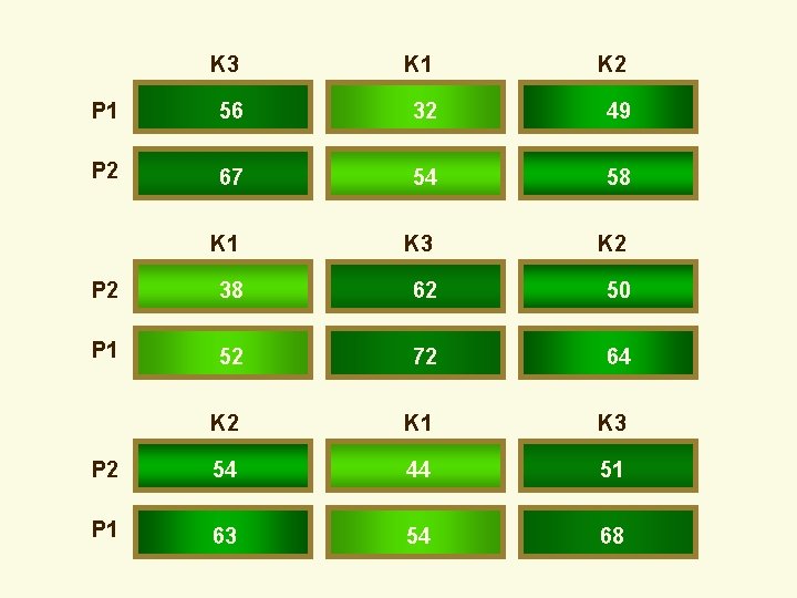
K 3 K 1 K 2 P 1 56 32 49 P 2 67 54 58 K 1 K 3 K 2 P 2 38 62 50 P 1 52 72 64 K 2 K 1 K 3 P 2 54 44 51 P 1 63 54 68

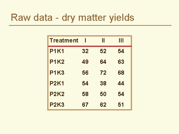
Raw data - dry matter yields Treatment I II III P 1 K 1 32 52 54 P 1 K 2 49 64 63 P 1 K 3 56 72 68 P 2 K 1 54 38 44 P 2 K 2 58 50 54 P 2 K 3 67 62 51

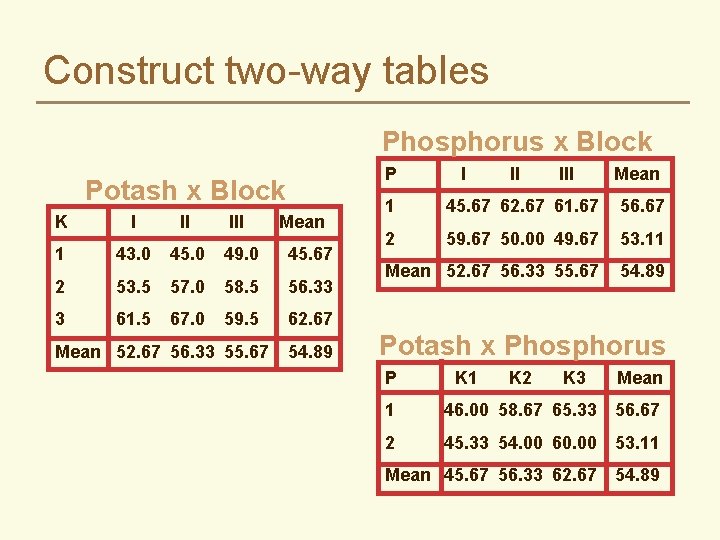
Construct two-way tables Phosphorus x Block P Potash x Block K I II III 1 43. 0 45. 0 49. 0 45. 67 2 53. 5 57. 0 58. 5 56. 33 3 61. 5 67. 0 59. 5 62. 67 Mean 52. 67 56. 33 55. 67 Mean 54. 89 I II III Mean 1 45. 67 62. 67 61. 67 56. 67 2 59. 67 50. 00 49. 67 53. 11 Mean 52. 67 56. 33 55. 67 54. 89 Potash x Phosphorus P K 1 K 2 K 3 Mean 1 46. 00 58. 67 65. 33 56. 67 2 45. 33 54. 00 60. 00 53. 11 Mean 45. 67 56. 33 62. 67 54. 89

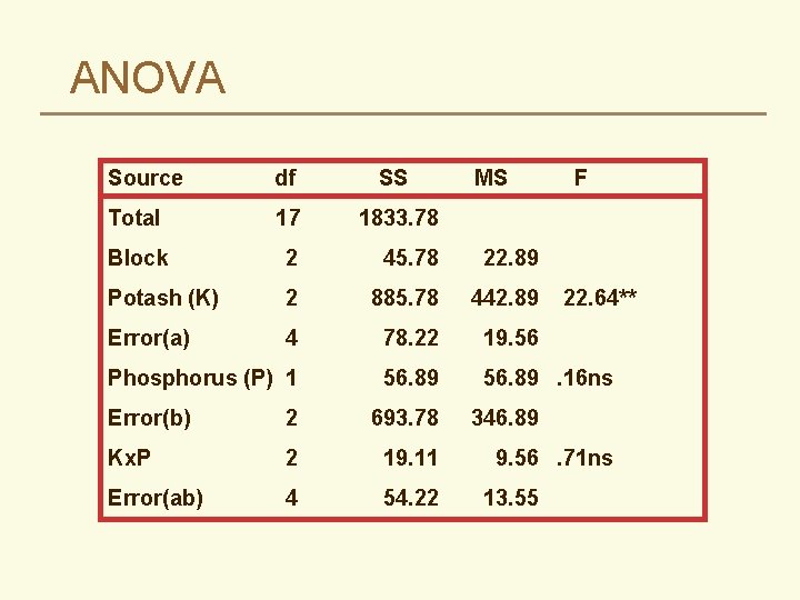
ANOVA Source df SS Total 17 1833. 78 Block 2 45. 78 22. 89 Potash (K) 2 885. 78 442. 89 Error(a) 4 78. 22 19. 56 Phosphorus (P) 1 56. 89. 16 ns Error(b) 2 693. 78 Kx. P 2 19. 11 Error(ab) 4 54. 22 MS F 22. 64** 346. 89 9. 56. 71 ns 13. 55

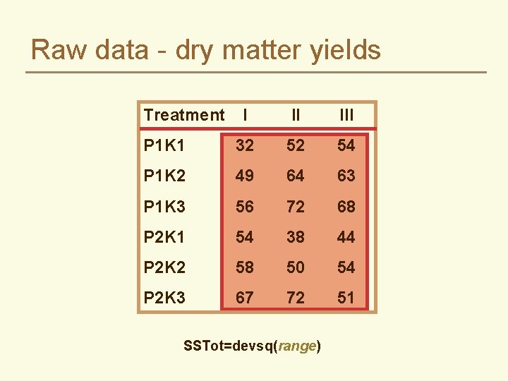
Raw data - dry matter yields Treatment I II III P 1 K 1 32 52 54 P 1 K 2 49 64 63 P 1 K 3 56 72 68 P 2 K 1 54 38 44 P 2 K 2 58 50 54 P 2 K 3 67 72 51 SSTot=devsq(range)

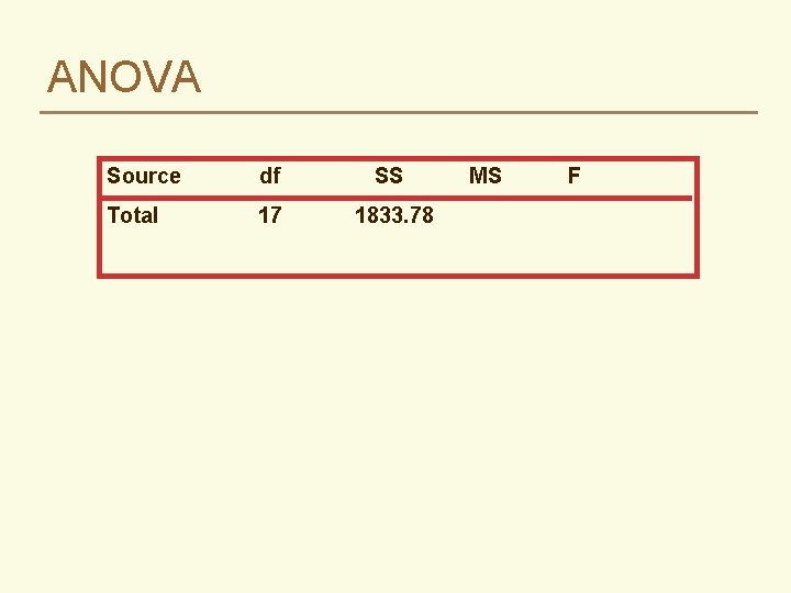
ANOVA Source df SS Total 17 1833. 78 MS F

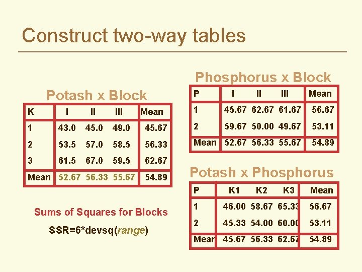
Construct two-way tables Phosphorus x Block Potash x Block P I II III Mean 1 45. 67 62. 67 61. 67 56. 67 45. 67 2 59. 67 50. 00 49. 67 53. 11 58. 5 56. 33 Mean 52. 67 56. 33 55. 67 54. 89 59. 5 62. 67 K I II III 1 43. 0 45. 0 49. 0 2 53. 5 57. 0 3 61. 5 67. 0 Mean 52. 67 56. 33 55. 67 Mean 54. 89 Potash x Phosphorus P Sums of Squares for Blocks SSR=6*devsq(range) K 1 K 2 K 3 Mean 1 46. 00 58. 67 65. 33 56. 67 2 45. 33 54. 00 60. 00 53. 11 Mean 45. 67 56. 33 62. 67 54. 89

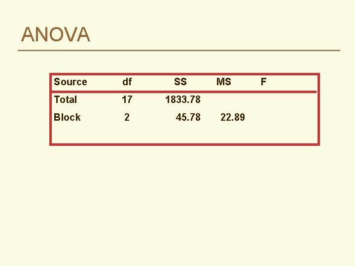
ANOVA Source df SS Total 17 1833. 78 Block 2 45. 78 MS 22. 89 F

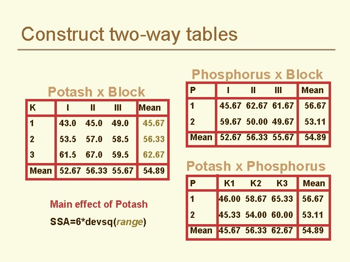
Construct two-way tables Phosphorus x Block Potash x Block P I II III Mean 1 45. 67 62. 67 61. 67 56. 67 45. 67 2 59. 67 50. 00 49. 67 53. 11 58. 5 56. 33 Mean 52. 67 56. 33 55. 67 54. 89 59. 5 62. 67 K I II III 1 43. 0 45. 0 49. 0 2 53. 5 57. 0 3 61. 5 67. 0 Mean 52. 67 56. 33 55. 67 Mean 54. 89 Potash x Phosphorus P Main effect of Potash SSA=6*devsq(range) K 1 K 2 K 3 Mean 1 46. 00 58. 67 65. 33 56. 67 2 45. 33 54. 00 60. 00 53. 11 Mean 45. 67 56. 33 62. 67 54. 89

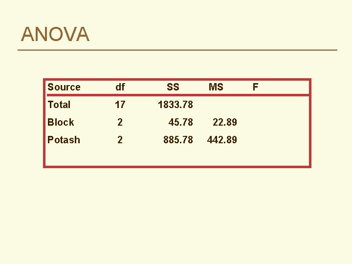
ANOVA Source df SS MS Total 17 1833. 78 Block 2 45. 78 22. 89 Potash 2 885. 78 442. 89 F

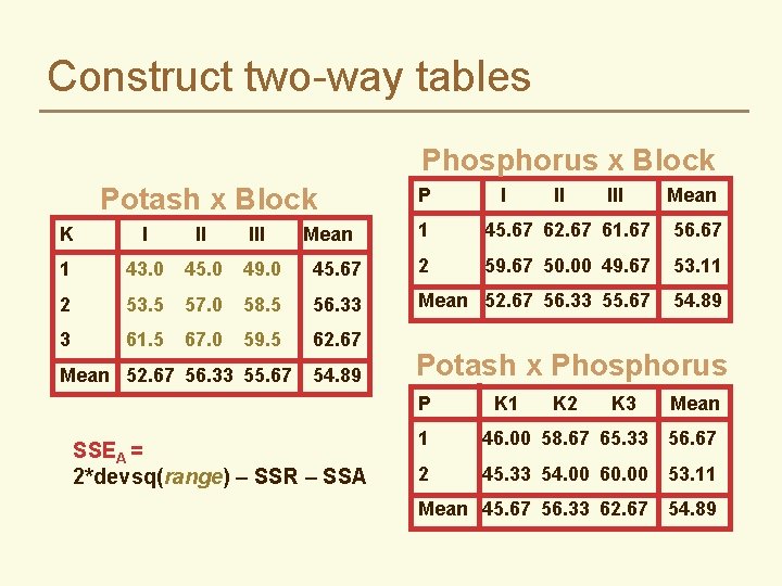
Construct two-way tables Phosphorus x Block Potash x Block P I II III Mean 1 45. 67 62. 67 61. 67 56. 67 45. 67 2 59. 67 50. 00 49. 67 53. 11 58. 5 56. 33 Mean 52. 67 56. 33 55. 67 54. 89 59. 5 62. 67 K I II III 1 43. 0 45. 0 49. 0 2 53. 5 57. 0 3 61. 5 67. 0 Mean 52. 67 56. 33 55. 67 Mean 54. 89 Potash x Phosphorus P SSEA = 2*devsq(range) – SSR – SSA K 1 K 2 K 3 Mean 1 46. 00 58. 67 65. 33 56. 67 2 45. 33 54. 00 60. 00 53. 11 Mean 45. 67 56. 33 62. 67 54. 89

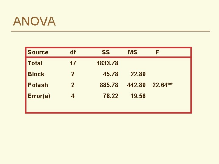
ANOVA Source df SS MS Total 17 1833. 78 Block 2 45. 78 22. 89 Potash 2 885. 78 442. 89 Error(a) 4 78. 22 19. 56 F 22. 64**

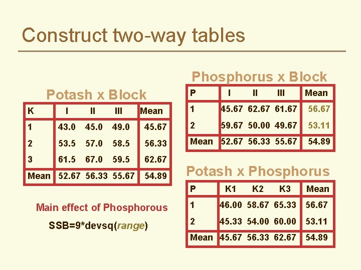
Construct two-way tables Phosphorus x Block Potash x Block P I II III Mean 1 45. 67 62. 67 61. 67 56. 67 45. 67 2 59. 67 50. 00 49. 67 53. 11 58. 5 56. 33 Mean 52. 67 56. 33 55. 67 54. 89 59. 5 62. 67 K I II III 1 43. 0 45. 0 49. 0 2 53. 5 57. 0 3 61. 5 67. 0 Mean 52. 67 56. 33 55. 67 Mean 54. 89 Potash x Phosphorus P Main effect of Phosphorous SSB=9*devsq(range) K 1 K 2 K 3 Mean 1 46. 00 58. 67 65. 33 56. 67 2 45. 33 54. 00 60. 00 53. 11 Mean 45. 67 56. 33 62. 67 54. 89

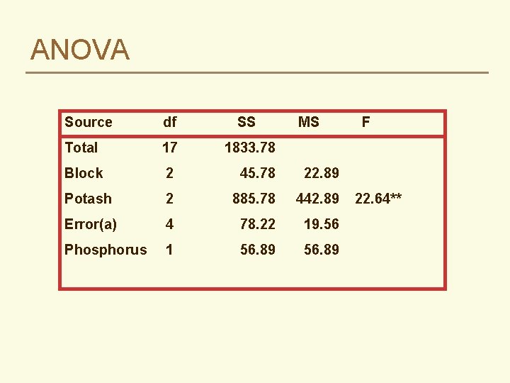
ANOVA Source df SS MS Total 17 1833. 78 Block 2 45. 78 22. 89 Potash 2 885. 78 442. 89 Error(a) 4 78. 22 19. 56 Phosphorus 1 56. 89 F 22. 64**

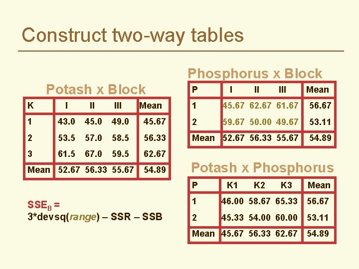
Construct two-way tables Phosphorus x Block Potash x Block K I II III 1 43. 0 45. 0 49. 0 2 53. 5 57. 0 3 61. 5 67. 0 Mean P I II III Mean 1 45. 67 62. 67 61. 67 56. 67 45. 67 2 59. 67 50. 00 49. 67 53. 11 58. 5 56. 33 Mean 52. 67 56. 33 55. 67 54. 89 59. 5 62. 67 Mean 52. 67 56. 33 55. 67 54. 89 Potash x Phosphorus P SSEB = 3*devsq(range) – SSR – SSB K 1 K 2 K 3 Mean 1 46. 00 58. 67 65. 33 56. 67 2 45. 33 54. 00 60. 00 53. 11 Mean 45. 67 56. 33 62. 67 54. 89

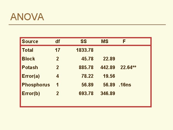
ANOVA Source df SS MS Total 17 1833. 78 Block 2 45. 78 22. 89 Potash 2 885. 78 442. 89 Error(a) 4 78. 22 19. 56 Phosphorus 1 56. 89. 16 ns Error(b) 2 693. 78 346. 89 F 22. 64**

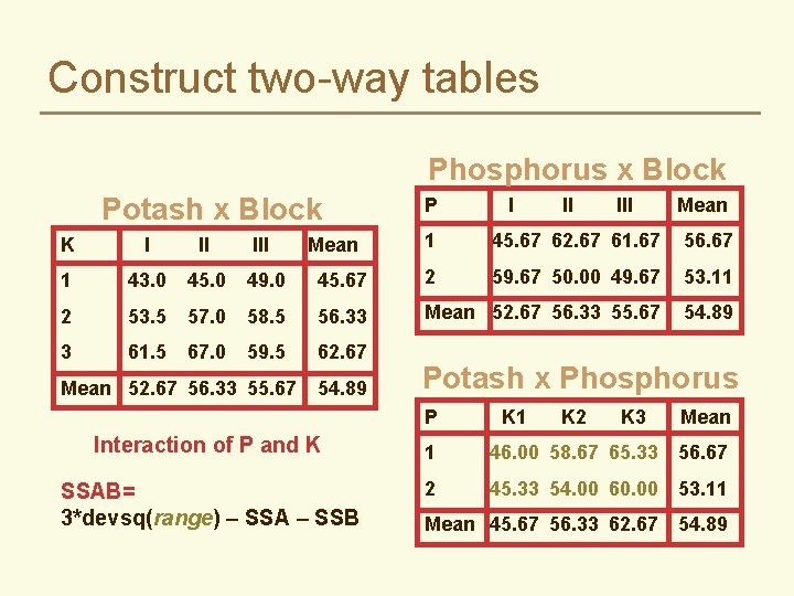
Construct two-way tables Phosphorus x Block Potash x Block P I II III Mean 1 45. 67 62. 67 61. 67 56. 67 45. 67 2 59. 67 50. 00 49. 67 53. 11 58. 5 56. 33 Mean 52. 67 56. 33 55. 67 54. 89 59. 5 62. 67 K I II III 1 43. 0 45. 0 49. 0 2 53. 5 57. 0 3 61. 5 67. 0 Mean 52. 67 56. 33 55. 67 Mean 54. 89 Potash x Phosphorus P K 1 K 2 K 3 Mean Interaction of P and K 1 46. 00 58. 67 65. 33 56. 67 SSAB= 3*devsq(range) – SSA – SSB 2 45. 33 54. 00 60. 00 53. 11 Mean 45. 67 56. 33 62. 67 54. 89

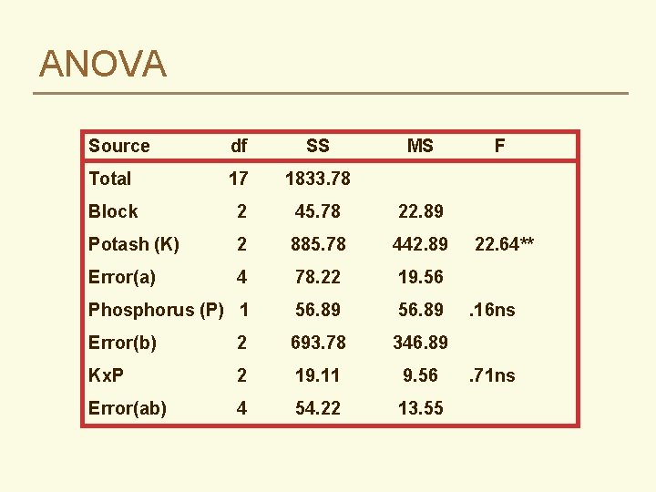
ANOVA Source df SS MS Total 17 1833. 78 Block 2 45. 78 22. 89 Potash (K) 2 885. 78 442. 89 Error(a) 4 78. 22 19. 56 Phosphorus (P) 1 56. 89 Error(b) 2 693. 78 346. 89 Kx. P 2 19. 11 9. 56 Error(ab) 4 54. 22 13. 55 F 22. 64**. 16 ns. 71 ns

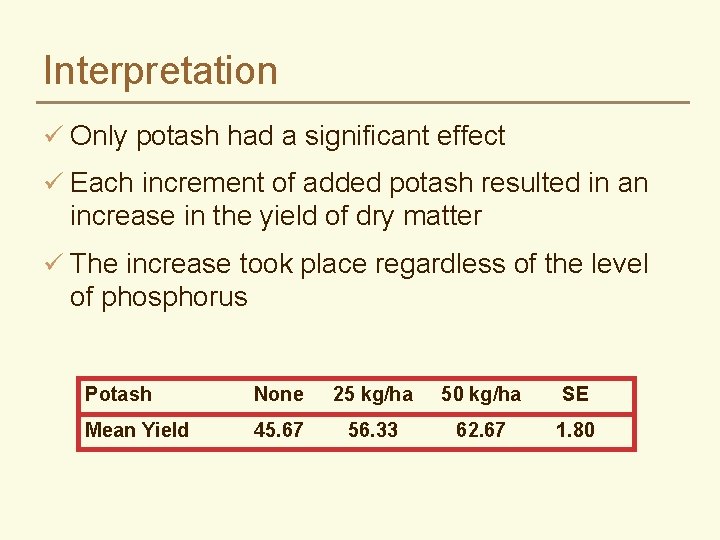
Interpretation ü Only potash had a significant effect ü Each increment of added potash resulted in an increase in the yield of dry matter ü The increase took place regardless of the level of phosphorus Potash None 25 kg/ha 50 kg/ha SE Mean Yield 45. 67 56. 33 62. 67 1. 80

Repeated measurements over time ü We often wish to take repeated measures on experimental units to observe trends in response over time. – repeated cuttings of a pasture – multiple observations on the same animal (developmental responses) ü Often provides more efficient use of resources than using different experimental units for each time period ü May also provide more precise estimation of time trends by reducing random error among experimental units – effect is similar to blocking ü Problem: observations over time are not assigned at random to experimental units. – Observations on the same plot will tend to be positively correlated – Correlations are greatest for samples taken at short time intervals and less for distant sampling periods

Repeated measurements over time ü The simplest approach is to treat sampling times as sub- plots in a split-plot experiment. – Some references recommend use of strip-plot rather than splitplot – This is valid only if all pairs of sub-plots in each main plot can be assumed to be equally correlated. • Compound symmetry • Sphericity ü Univariate adjustments can be made ü Multivariate procedures can be used to adjust for the correlations among sampling periods

Univariate adjustments for repeated measures ü Reduce df for subplots, interactions, and subplot error terms to obtain more conservative F tests ü Fit a smooth curve to the time trends and analyze a derived variable – – average maximum response area under curve time to reach the maximum ü Use polynomial contrasts to evaluate trends over time (linear, quadratic responses) and compare responses for each treatment – Can be done with the REPEATED statement in PROC GLM

Multivariate adjustments for repeated measures ü Stage one: estimate covariance structure for residuals ü Stage two: – include covariance structure in the model – use generalized least squares methodology to evaluate treatment and time effects ü Computer intensive – use PROC MIXED or GLIMMIX in SAS Reference: Littell et al. , 2002. SAS for Linear Models, Chapter 8.