Streaming Pattern Discovery in Multiple TimeSeries Spiros Papadimitriou

Streaming Pattern Discovery in Multiple Time-Series Spiros Papadimitriou Jimeng Sun Christos Faloutsos Carnegie Mellon University VLDB 2005, Trondheim, Norway

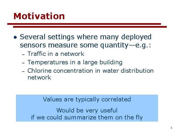
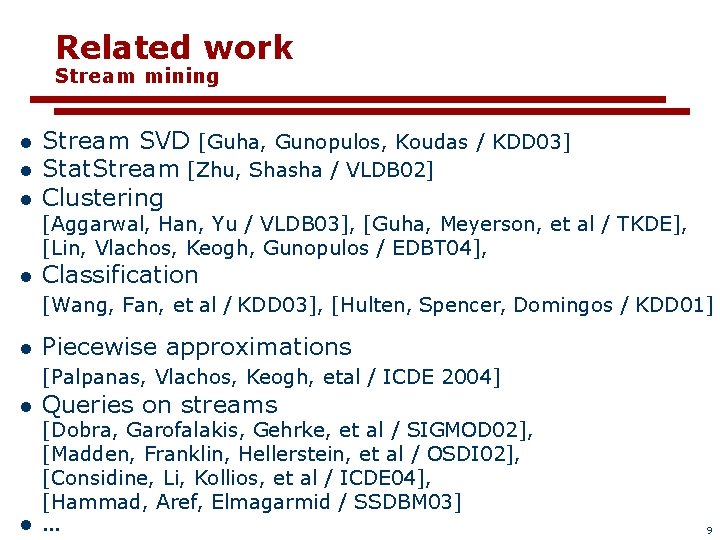
Motivation l Several settings where many deployed sensors measure some quantity—e. g. : – – – Traffic in a network Temperatures in a large building Chlorine concentration in water distribution network Values are typically correlated Would be very useful if we could summarize them on the fly 2

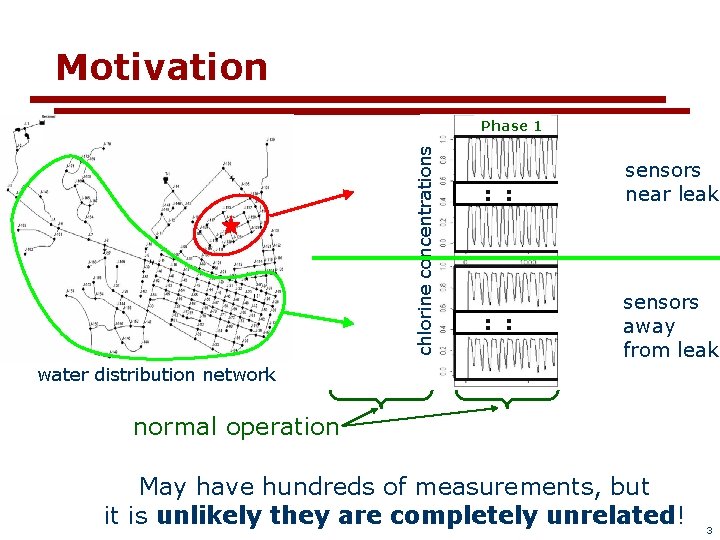
Motivation chlorine concentrations Phase 1 : : Phase 2 Phase 3 sensors : : near leak : : sensors : : away : : from leak water distribution network normal operation May have hundreds of measurements, but it is unlikely they are completely unrelated! 3

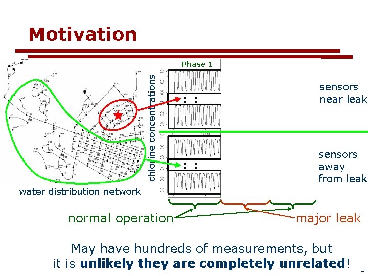
Motivation chlorine concentrations Phase 1 : : Phase 2 : : Phase 3 : : sensors near leak sensors away from leak water distribution network normal operation major leak May have hundreds of measurements, but it is unlikely they are completely unrelated! 4

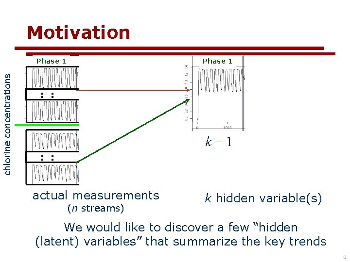
Motivation chlorine concentrations Phase 1 : : k=1 : : actual measurements (n streams) k hidden variable(s) We would like to discover a few “hidden (latent) variables” that summarize the key trends 5

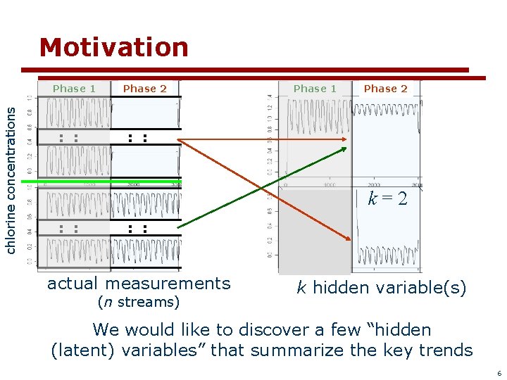
Motivation chlorine concentrations Phase 1 : : Phase 2 : : Phase 1 Phase 2 : : k=2 : : actual measurements (n streams) k hidden variable(s) We would like to discover a few “hidden (latent) variables” that summarize the key trends 6

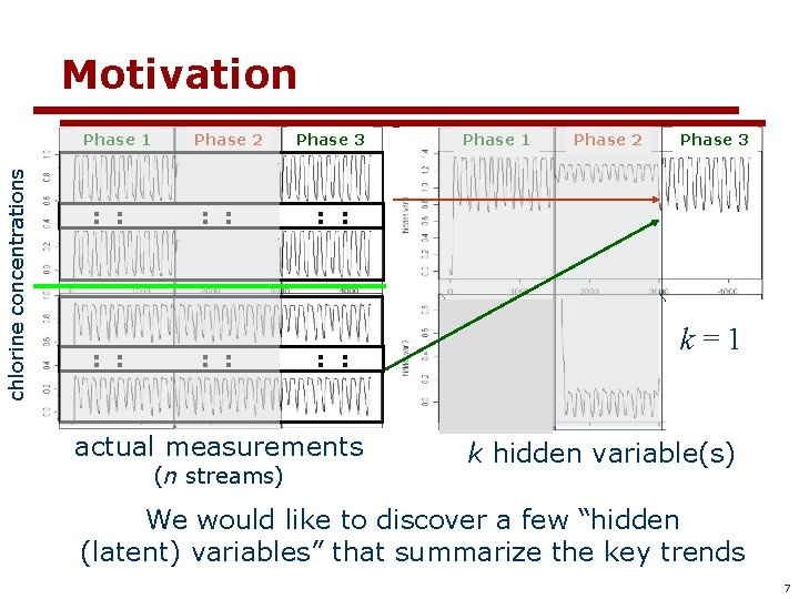
Motivation chlorine concentrations Phase 1 : : Phase 2 : : Phase 3 Phase 2 Phase 3 : : actual measurements (n streams) Phase 1 k=1 k hidden variable(s) We would like to discover a few “hidden (latent) variables” that summarize the key trends 7

Goals l Discover “hidden” (latent) variables for: – – l l Summarization of main trends for users Efficient forecasting, spotting outliers/anomalies Incremental, real-time computation Limited memory requirements 8

Related work Stream mining l l l Stream SVD [Guha, Gunopulos, Koudas / KDD 03] Stat. Stream [Zhu, Shasha / VLDB 02] Clustering [Aggarwal, Han, Yu / VLDB 03], [Guha, Meyerson, et al / TKDE], [Lin, Vlachos, Keogh, Gunopulos / EDBT 04], l Classification [Wang, Fan, et al / KDD 03], [Hulten, Spencer, Domingos / KDD 01] l Piecewise approximations [Palpanas, Vlachos, Keogh, etal / ICDE 2004] l Queries on streams [Dobra, Garofalakis, Gehrke, et al / SIGMOD 02], [Madden, Franklin, Hellerstein, et al / OSDI 02], [Considine, Li, Kollios, et al / ICDE 04], [Hammad, Aref, Elmagarmid / SSDBM 03] l … 9

Overview l l Method outline Experiments 10

Stream correlations l Step 1: How to capture correlations? l Step 2: How to do it incrementally, when we have a very large number of points? l Step 3: How to dynamically adjust the number of hidden variables? 11

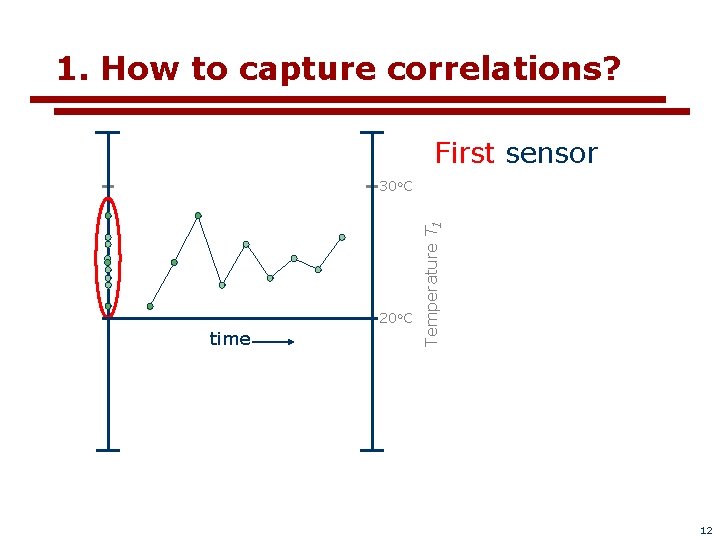
1. How to capture correlations? First sensor 20 o. C time Temperature T 1 30 o. C 12

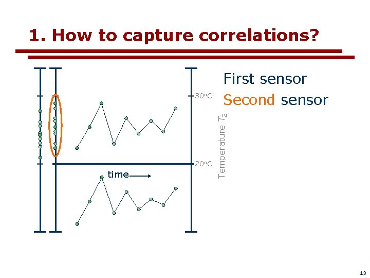
1. How to capture correlations? 20 o. C time Temperature T 2 30 o. C First sensor Second sensor 13

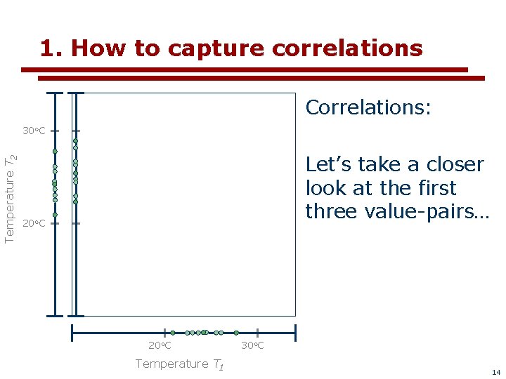
1. How to capture correlations Correlations: Temperature T 2 30 o. C Let’s take a closer look at the first three value-pairs… 20 o. C Temperature T 1 30 o. C 14

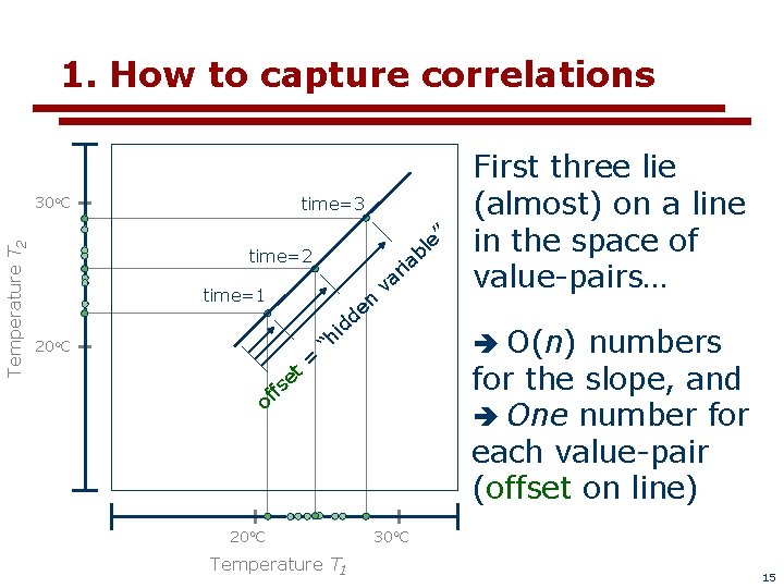
1. How to capture correlations time=3 Temperature T 2 30 o. C ” time=2 time=1 n e d ia r va d 20 o. C t e s = i “h Temperature T 1 O(n) numbers for the slope, and One number for each value-pair (offset on line) f of 20 o. C e bl First three lie (almost) on a line in the space of value-pairs… 30 o. C 15

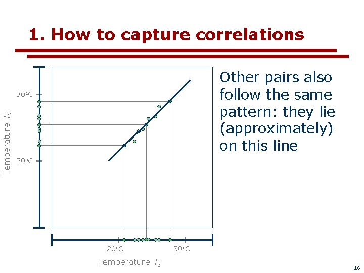
1. How to capture correlations Other pairs also follow the same pattern: they lie (approximately) on this line Temperature T 2 30 o. C 20 o. C Temperature T 1 30 o. C 16

Stream correlations l Step 1: How to capture correlations? l Step 2: How to do it incrementally, when we have a very large number of points? l Step 3: How to dynamically adjust the number of hidden variables? 17

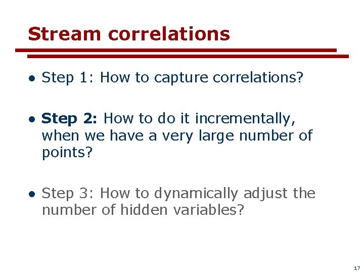
2. Incremental update Temperature T 2 30 o. C For each new point l Project onto current line l Estimate error 20 o. C Temperature T 1 30 o. C New value 18

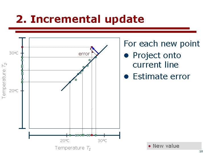
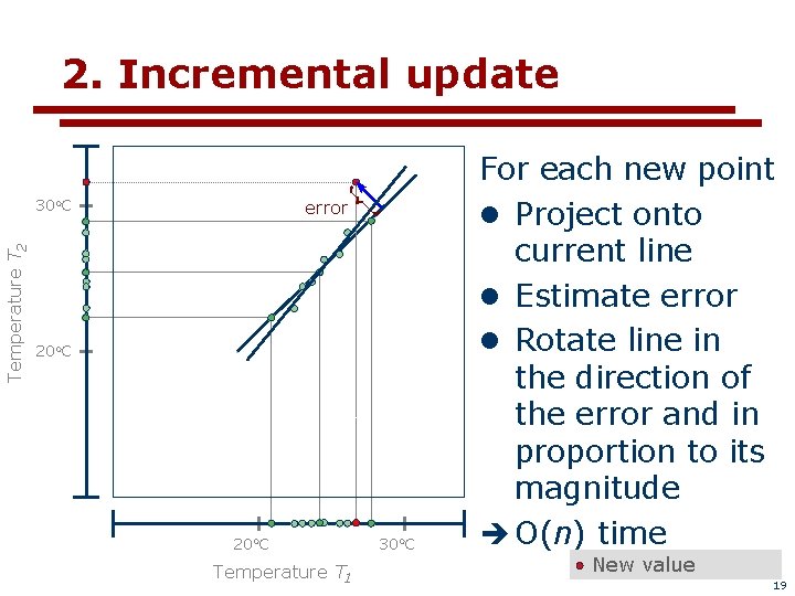
2. Incremental update Temperature T 2 30 o. C error 20 o. C Temperature T 1 30 o. C For each new point l Project onto current line l Estimate error l Rotate line in the direction of the error and in proportion to its magnitude O(n) time New value 19

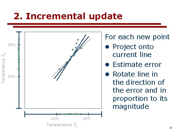
2. Incremental update For each new point l Project onto current line l Estimate error l Rotate line in the direction of the error and in proportion to its magnitude Temperature T 2 30 o. C 20 o. C Temperature T 1 30 o. C 20

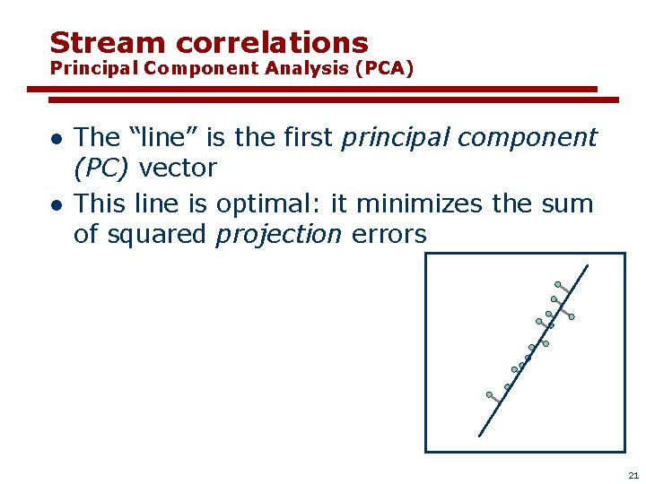
Stream correlations Principal Component Analysis (PCA) l l The “line” is the first principal component (PC) vector This line is optimal: it minimizes the sum of squared projection errors 21

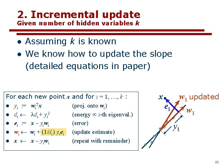
2. Incremental update Given number of hidden variables k l l Assuming k is known We know how to update the slope (detailed equations in paper) For each new point x and for i = 1, …, k : l yi : = wi. Tx (proj. onto wi) l di + yi 2 (energy i-th eigenval. ) l ei : = x – yiwi (error) l wi + (1/di) yiei (update estimate) l x x – yiwi (repeat with remainder) x e 1 w 1 updated w 1 y 1 22

Stream correlations l Step 1: How to capture correlations? l Step 2: How to do it incrementally, when we have a very large number of points? l Step 3: How to dynamically adjust k, the number of hidden variables? 23

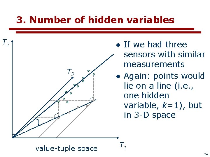
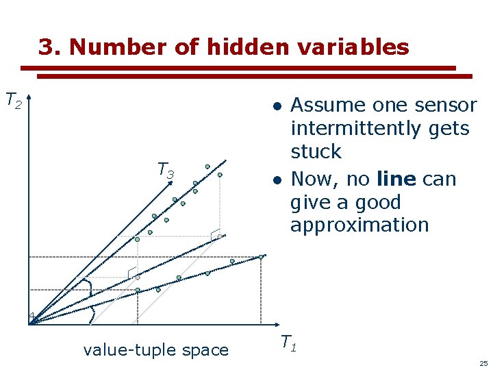
3. Number of hidden variables T 2 l T 3 value-tuple space l If we had three sensors with similar measurements Again: points would lie on a line (i. e. , one hidden variable, k=1), but in 3 -D space T 1 24

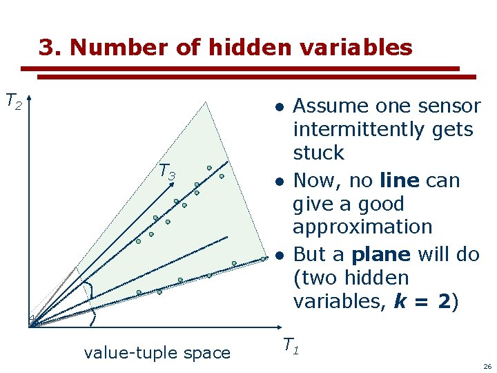
3. Number of hidden variables T 2 l T 3 value-tuple space l Assume one sensor intermittently gets stuck Now, no line can give a good approximation T 1 25

3. Number of hidden variables T 2 l T 3 l l value-tuple space Assume one sensor intermittently gets stuck Now, no line can give a good approximation But a plane will do (two hidden variables, k = 2) T 1 26

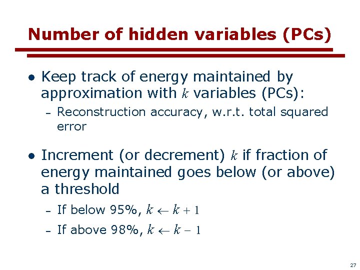
Number of hidden variables (PCs) l Keep track of energy maintained by approximation with k variables (PCs): – l Reconstruction accuracy, w. r. t. total squared error Increment (or decrement) k if fraction of energy maintained goes below (or above) a threshold – If below 95%, k k 1 – If above 98%, k k 1 27

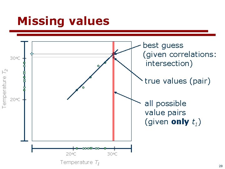
Missing values best guess (given correlations: intersection) Temperature T 2 30 o. C true values (pair) 20 o. C all possible value pairs (given only t 1) 20 o. C Temperature T 1 30 o. C 28

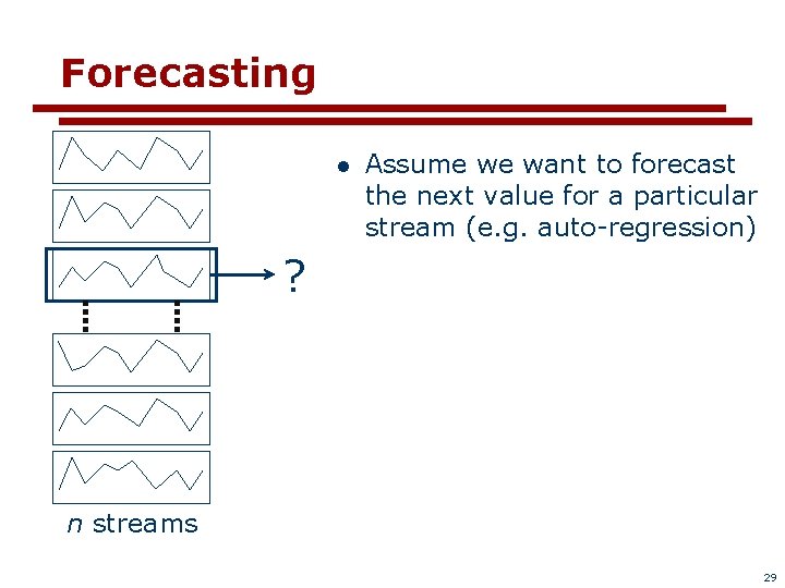
Forecasting l Assume we want to forecast the next value for a particular stream (e. g. auto-regression) ? n streams 29

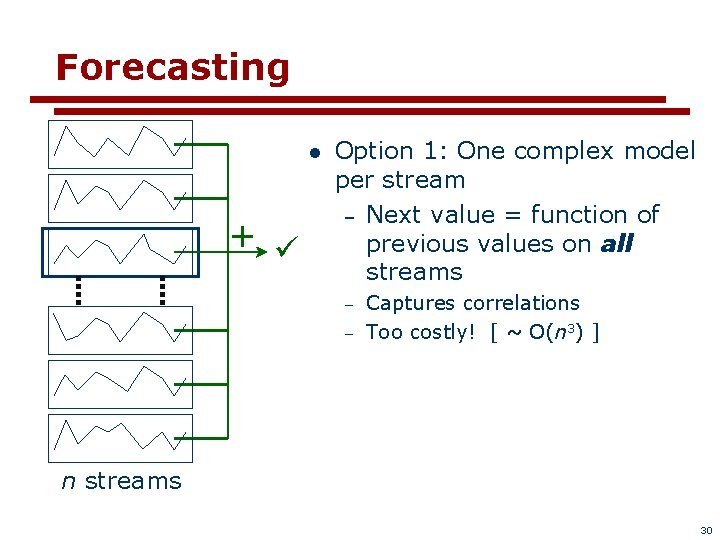
Forecasting l + Option 1: One complex model per stream – Next value = function of previous values on all streams – – Captures correlations Too costly! [ ~ O(n 3) ] n streams 30

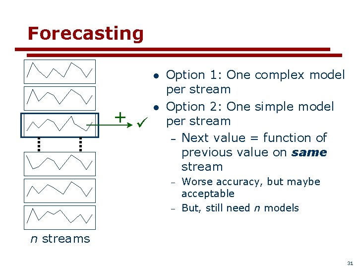
Forecasting l + l Option 1: One complex model per stream Option 2: One simple model per stream – Next value = function of previous value on same stream – – Worse accuracy, but maybe acceptable But, still need n models n streams 31

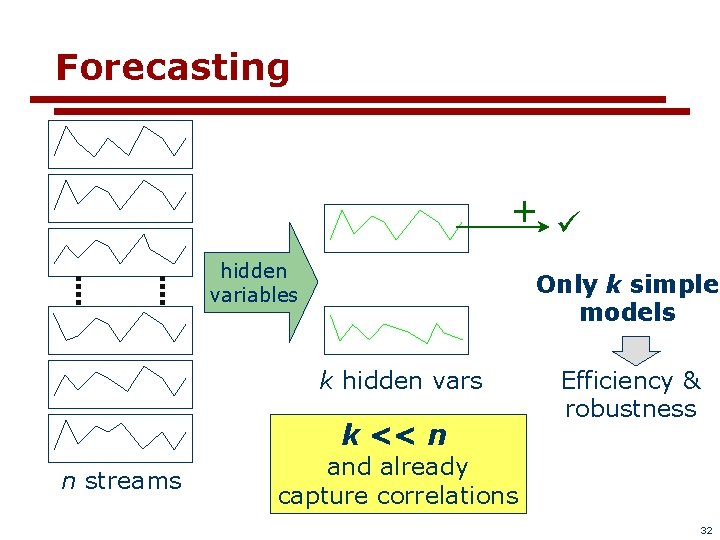
Forecasting + hidden variables Only k simple models k hidden vars k << n n streams Efficiency & robustness and already capture correlations 32

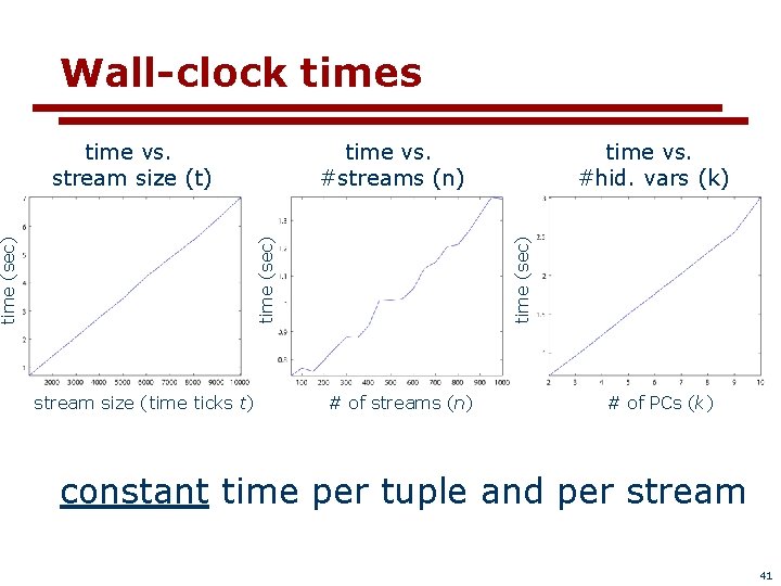
Time/space requirements Incremental PCA O(nk) space (total) and time (per tuple), i. e. , l Independent of # points (t) l Linear w. r. t. # streams (n) l Linear w. r. t. # hidden variables (k) In fact, l Can be done in real time [demo] 33

Overview l l Method outline Experiments 34

Experiments Chlorine concentration Measurements Reconstruction [CMU Civil Engineering] 166 streams 2 hidden variables (~4% error) 35

Experiments Chlorine concentration hidden variables l l l [CMU Civil Engineering] Both capture global, periodic pattern Second: ~ first, but “phase-shifted” Can express any “phase-shift”… 36

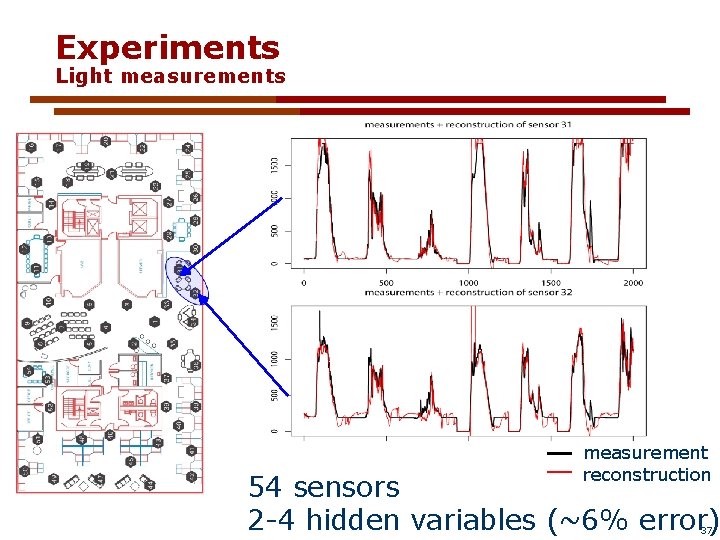
Experiments Light measurements measurement reconstruction 54 sensors 2 -4 hidden variables (~6% error) 37

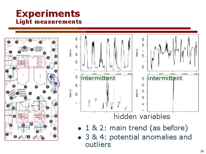
Experiments Light measurements intermittent hidden variables l l 1 & 2: main trend (as before) 3 & 4: potential anomalies and outliers 38

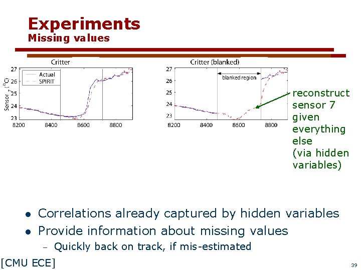
Experiments Missing values reconstruct sensor 7 given everything else (via hidden variables) l l Correlations already captured by hidden variables Provide information about missing values – Quickly back on track, if mis-estimated [CMU ECE] 39

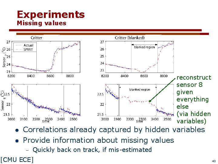
Experiments Missing values reconstruct sensor 8 given everything else (via hidden variables) l l Correlations already captured by hidden variables Provide information about missing values – Quickly back on track, if mis-estimated [CMU ECE] 40

Wall-clock times time (sec) stream size (time ticks t) time vs. #hid. vars (k) time (sec) time vs. #streams (n) time (sec) time vs. stream size (t) # of streams (n) # of PCs (k) constant time per tuple and per stream 41

Conclusion l Many settings with hundreds of streams, but – Stream values are, by nature, related – In reality, there are only a few variables Discover hidden variables for – – Summarization of main trends for users Efficient forecasting, spotting outliers/anomalies Incremental, real time computation With limited memory 42

End Thank you 43