Stream Measures Engineering view of a stream 1

Stream Measures

Engineering view of a stream 1 5 V = 2 m/s A = 3 m 2 n = 0. 04 t = 120 N/m 2 Ecological view of a stream B-IBI = 23 p. H = 7. 2 TDS = 110 mg/l DO = 8. 3 mg/l D 50 = 10 cm Adapted from Gordon et al. 1992

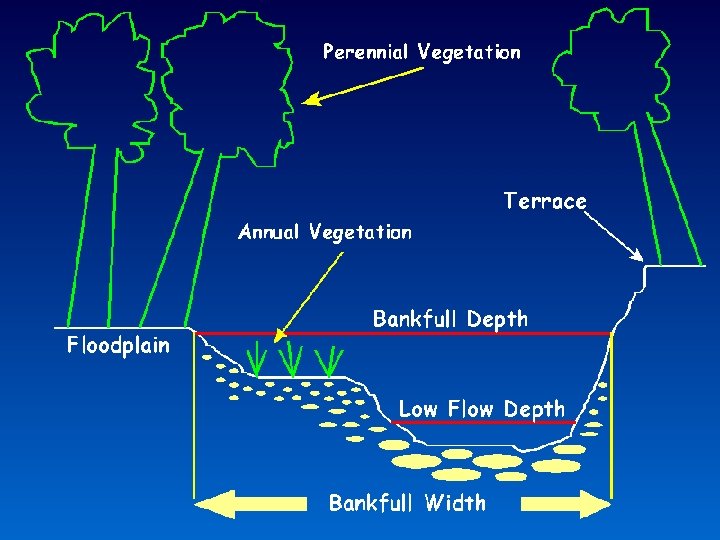
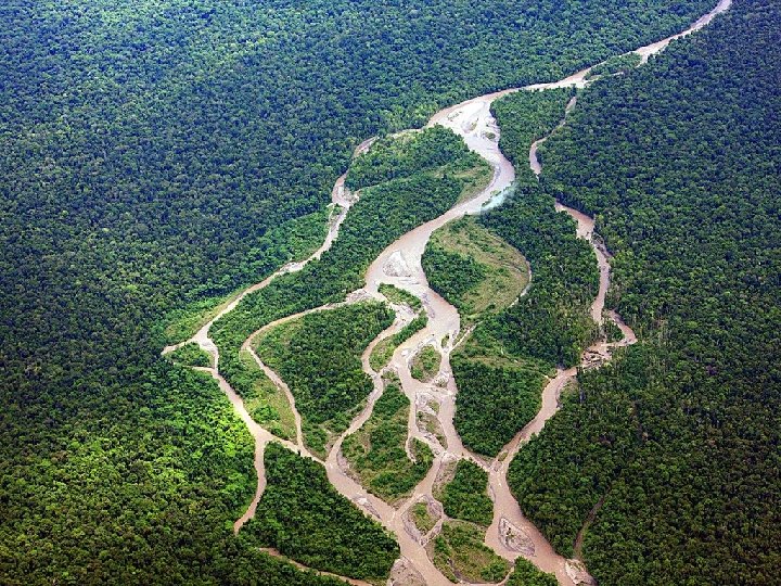
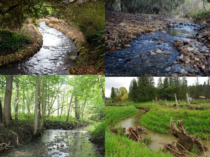
Geomorphology

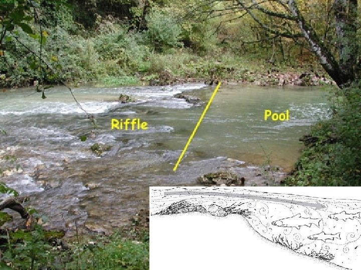
Pools, Riffle, & Glides

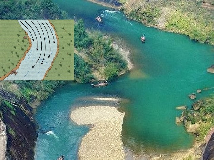
Velocity Distribution In A Channel

Vertical dimensions • Velocity changes with depth in stream channel Diagram by: Eric G. Paterson, Department of Mechanical and Nuclear Engineering, The Pennsylvania State University

Velocity Profile 0. 2 0. 6 depth 0. 8 If stream is deep, take average of measurements at 0. 2 and 0. 8

How do we measure how much water is in a stream? • Volumetric measurements– Works for very low flows, collect a known volume of water for a known period of time Volume/time is discharge = Q • Cross-section/velocity measurements – Velocity Area – Float Method • Dilution gaging with salt or dye • Artificial controls like weirs • Empirical equations, e. g. Manning’s eqn.

Site factors for gaging 1. stable control - bedrock, non-erosive channel, man-made structure 2. locate gage a short distance above control 3. want minimal backwater or tidal influence 4. straight reach above gage for 4 -5 channel widths 5. No local inflows or outflows- groundwater or flood bypasses 6. must be accessible at all times 7. securely mounted structure 8. stable confining banks 9. good to have a benchmark nearby for datum 10. good to have an auxiliary stage nearby- staff gage

Other considerations • • Few eddies or areas of zero velocity Few instream obstacles Relatively consistent cross-section profile Velocity and depth do not exceed instrument capabilities or personnel height

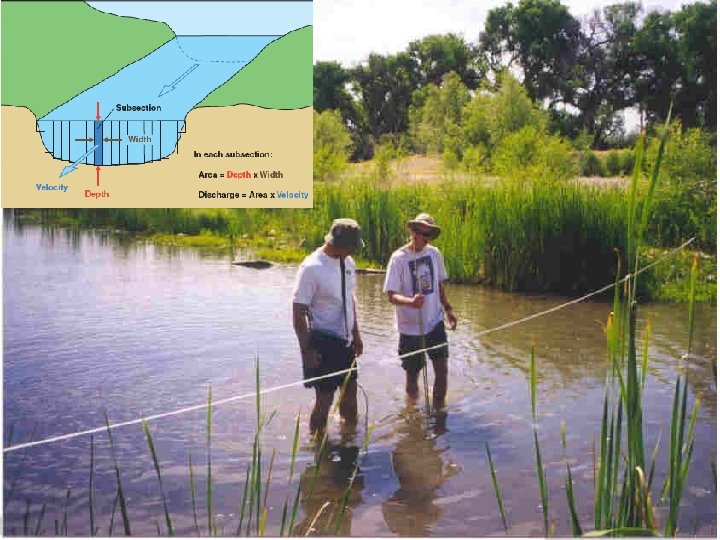
Velocity – Area discharge measurement method By measuring the cross-sectional area of the stream and the water velocity you can compute discharge Q = VA Q = discharge Where Q is discharge V is velocity A is wetted cross-sectional area and depth = width x depth units are ft 3/s or L 3/t (volume / time) This is a continuity of mass equation A * V = Q = A* V Q stays constant unless you add more water

Pygmy Meter Rotations make clicking sound in headphones Swoffer Meter Spinning meters need to overcome friction – increases error to some degree If current strong may need weight

How many subsections? • Subsections should be at least 0. 3 feet or ~0. 1 m wide • Each subsection should have 10% or less of total discharge • Number of subsections should be doable in a reasonable amount of time

Velocity – Area method of discharge measurement Tape measure- horizontal location of measures taken from tape Water surface Measurement represents mid-section of a polygon Velocity measured 0. 6 d from water surface (0. 4 d from bottom) Record x value (tape distance), y value (total depth at measurement site) v, velocity at depth 0. 6 d from top (staff will do this for you)

Mid-point method of calculating discharge (Q) Location of depth and velocity measurements Area included Area not included Key Assumption: Over estimation (area included) = Under estimation (area not included), therefore cross-section area is simply the sum of all the sections (rectangles), which is much easier than taking the integral! However, the hypotenuse of each over-under estimation triangle can be used to calculate the wetted perimeter.

Equation for computing subsection discharge - qi Equation for computing q in each subsection X = distance of each velocity point along tape Y = depth of flow where velocity is measured V = velocity Q = total discharge = sum of qis

How Calcs work week 1 Enter velocity meter data in the yellow boxes Method: Site: velocity meter Date: 1/14/16 Data enterer: Marisa Bass Weather: Sunny, no precip. Location on tape (feet) Depth (feet) (X) (Y) Left Edge water Right Edge water Lower watershed 5. 8 Time: 1: 10 p. m. Team: 4 Area Velocity @ 0. 6 D Q Interval (ft 2) fps (ft 3)/s 0. 0 0 0. 00 0 6. 7 0. 35 0. 2625 0. 17 0. 044625 7. 3 0. 55 0. 3575 0. 24 0. 0858 8. 0 0. 45 0. 3375 0. 32 0. 108 8. 8 0. 42 0. 294 0. 41 0. 12054 9. 4 0. 0 0 0. 00 0 Comments: Q Total = Water level 0. 6 ft below high water mark on right side of bank. 0. 36

week 1 Enter velocity meter data in the yellow boxes Method: Site: velocity meter Date: 1/14/16 Data enterer: Marisa Bass Weather: Sunny, no precip. Left Edge water Lower watershed Comments: 1: 10 p. m. Team: 4 Q Interval (ft 3)/s Location on tape (feet) Depth (feet) Area Velocity @ 0. 6 D Cell number (X) (Y) (ft 2) fps 1 2 5. 8 6. 7 0. 0 0. 35 0 A 2= (X 3 -X 1 / 2) * Y 2 0. 00 0. 17 0 Q 2 = A 2 *V 2 3 7. 3 0. 55 A 3= (X 4 -X 2 / 2) * Y 3 0. 24 Q 3 = A 3 *V 3 4 8. 0 0. 45 A 4= (X 5 -X 3 / 2) * Y 4 0. 32 Q 4 = A 4 *V 4 5 8. 8 0. 42 A 5= (X 6 -X 4 / 2) * Y 5 0. 41 Q 5 = A 5 *V 5 0. 0 A 6= (X 7 -X 5 / 2) * Y 6 0 (note can use eq, but will zero out ) 6 Right Edge water Time: 7 9. 4 Q 6 = A 6 *V 6 0. 00 Q Total = 0 Sum all Qn

Float method of discharge measurement • Gives reasonable estimates when no equipment is available • Use something that floats that you can retrieve or is biodegradable if you can’t retrieve it – E. g. oranges, dried orange peels, tennis balls, leaves, twigs – You can float yourself as a last resort

Float method of discharge measurement correction factors • Area-velocity method measure velocity at 0. 6 d (= ave V) • Float method measures surface velocity (not ave V for column) • Need to correct to better estimate average subsurface velocity Q = A* Vsurf * velocity correction factor

Float Method surface velocity = distance / time average velocity = (k*surface velocity) U Mass, Boston

Dilution gaging method • Use a chemical tracer, dye or salt – Exotic to stream – Stable – Non-toxic – Cheap – Detectable • Do mass balance on concentrations upstream and downstream

How else might we estimate streamflow? Stream Stage- elevation The stage of a stream is the elevation of the water surface above a datum. The most commonly used datum is mean sea level. Gages are used to measure the stage of streams. Types of gages: - recording - non-recording

Fixed Gauging Stations - Weirs Stable cross section with simple geometry rating curve – just measure stage

How do we measure the stage? Nonrecording gauges Staff Gauge Estimating Peak Flow Debris Line U Mass, Boston Crest Gauges - Cork

Continuous Measurement - Water Level Recorders

The Stage of a Stream Float moves up / down with water surface

How can we relate stage to discharge? Rating Curve – relates stage to discharge Empirical relationship from observations Measure discharge at different flows USGS Rating curves usually have a break point, which is around the stage at which the river spreads out of it's banks, or it could be at a lower stage if the river bed cross section changes dramatically. Above that stage, the river does not rise as fast, given that other conditions remain constant. This is illustrated by a change in slope in the rating curve. On this figure the break point appears to be around 6 -7 feet.

Rating curve We can do this is Excel Very often it is a power equation (log-log) Fit a mathematical equation

Resistance Equations Manning’s Equation • In 1889 Irish Engineer, Robert Manning presented the formula: Equation 7. 2 • v is the flow velocity (ft/s) • n is known as Manning’s n and is a coefficient of roughness • R is the hydraulic radius (A/P) where P is the wetted perimeter (ft) • S is hydraulic grade line or water surface slope • If the water depth is constant, S is same as the channel bed slope • 1. 49 is a unit conversion factor. Approximated as 1. 5 in the book. Use 1. 0 if SI (metric) units are used.

Parameters for Manning’s equation Water surface Cross sectional area = A Wetted perimeter = p area of stream in contact with bottom and sides R = hydraulic radius = A/p

Table 7. 1 Manning’s n Roughness Coefficient Type of Channel and Description Minimum Normal Maximum Streams on a plain Clean, straight, full stage, no rifts or deep pools 0. 025 0. 033 Clean, winding, some pools, shoals, weeds & stones 0. 033 0. 045 0. 05 Same as above, lower stages and more stones 0. 045 0. 06 0. 05 0. 075 0. 15 Sluggish reaches, weedy, deep pools Very weedy reaches, deep pools, or floodways with heavy stand of timber and underbrush Mountain streams, no vegetation in channel, banks steep, trees & brush along banks submerged at high stages Bottom: gravels, cobbles, and few boulders 0. 03 0. 04 0. 05 Bottom: cobbles with large boulders 0. 04 0. 05 0. 07

http: //manningsn. sdsu. edu/barnes 013_24. html

Mountain Stream. Bottom with cobbles and large boulders http: //manningsn. sdsu. edu/barnes 101_41. html

Plains streamfull stage, no rifts or deep pools http: //manningsn. sdsu. edu/barnes 020_27. html

Table 7. 2. Values for the computation of the roughness coefficient (Chow, 1959) n = (n 0 + n 1 + n 2 + n 3 + n 4 ) m 5 Equation 7. 12