Stratigraphic Facies and Geologic Time Amantz Gressley 1834

Stratigraphic Facies and Geologic Time Amantz Gressley, 1834, and the Jurassic Rocks of the Jura Mountains between France and Switzerland

The Interpretation of Geologic History Requires Knowledge of the Following The Interpretation of Sedimentary Rocks Requires Knowledge of the Following: 1. Sedimentary Rocks 1. Rock Classification 2. Igneous Rocks 2. Depositional Environments 3. Metamorphic Rocks 3. Sedimentary Structures 4. Origin and History of Life 4. Sedimentary Tectonics 5. Tectonics, including: 5. Sedimentary Facies and Time • Structural geology • Plate tectonic theory • Etc. The core concept is tectonics since nothing in geology makes sense except in the light of tectonics

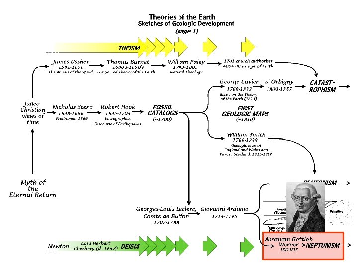
Abraham Gottlob Werner’s Geologic Time Scale The Neptunist World View Sea Level after deposition of the Primitive rocks Sea Level after deposition of the Transition rocks Stratified Sea Level after deposition of the Stratified rocks Transition Primitive Transported Primitive – crystalline rocks, both igneous and metamorphic. Thought to represent first chemical precipitates from a worldwide ocean. Transition – stony, indurated stratified rocks such as graywacke, limestones, sills. Stratified – obviously stratified fossiliferous rocks, thought to represent the first deposits after receding of the worldwide oceans, formed by erosion of emergent mountains. Transported – Poorly consolidated clays, sands and gravels. Thought to have been deposited after final withdrawal of a worldwide ocean. Volcanic – Younger lava flows associated with volcanic vents (added to the classification later as an afterthought, lavas were thought to be local phenomena resulting from the burning of coal beds.

Layer Cake Stratigraphy The study of rock strata, especially the distribution, deposition, and age of sedimentary rocks P 126 Werner’s theory made a firm prediction, that the same kinds of rocks should have been laid down in the same sequence all over the world.

The Facies Concept It is not certain who first noticed that rocks were not layer cake. Levoisier in 1789 is the earliest mention we have, but Amantz Gressley coined most of the important concepts while working in the Jura Mountains. While describing the rocks he observed lateral changes in the composition and described them with clarity calling these changes facies. But, then later in his paper he spoke of facies changes “in the vertical direction” meaning that the rocks were different vertically as well as horizontally. This has led to ongoing confusion. Perhaps a dozen different concepts and definitions about the facies have been proposed. But, they all go back to the two original ways Gressley used the term – his formal definition, and his offhanded use of the term.

Two Facies Definition One The facies is the sum total of all the physical, biological and chemical characteristics imparted to a sedimentary rock at the time of deposition. Definition Two Facies are the many different sediments and resulting rocks that form at the same time, but in different depositional environments.

The Transition from Wernerian "Transition Rocks" To the Lower Paleozoic Periods By Sedgewich and Murchinson, 1835 Sedgewick, 1835 Charles Lapworth 1879 Ordovician Cambrian Sedgewick, 1835 Cambrian overlap Opps ! Silurian Murchinson, 1835

Lyell 1833 Pleistocene Pliocene Miocene Eocene Gressley 1795 Cretaceous Jurassic Alberti 1834 Triassic D’Halloy 1822 Permian Williams 1891 Pennsylvan. Williams 1891 Mississippian Devonian Sedgewich & Murchinson 1839 Murchinson 1841 Murchinson 1835 Silurian Lapworth 1879 Ordovician Sedgewick 1835 Cambrian Carbonif. “Old Red ss” Unstudied Until 1830’s

The Transition from Wernerian "Transition Rocks" To the Lower Paleozoic Periods By Sedgewich and Murchinson Adapted from Dott and Batten: Evolution of the Earth

Old Red Sandstone Early Devonian fishes from the Old Red Sandstone of Spitzbergen (Wood Ray Formation) http: //www. picturescape. co. uk/gallery%20 pages /gallery%20 one/caldey%20 sandstone. htm http: //www. picturescape. co. uk/gallery%20 pages/gallery%20 one/caldey%20 sandstone. htm

Old Red Sandstone The Old Red Sandstone exhibited many changes over short distances, with thinly layered areas alternating with conglomerates and outstanding crossbedded sandstones. http: //virtual. yosemite. cc. ca. us/ghayes/Siccar%20 Point. htm

Devonian Marine Rocks of Devon, England The cliffs at Fremington are Devonian with Glacial beds on top of this, below the Devonian beds follows the carboniferous beds. Both Upper and Lower Carboniferous rocks have been found at Fremington, however it is suspected that some of these rocks have drifted from up or down stream, this could explain why occasionally blocks of Carboniferious limestone can be found. http: //www. ukfossils. co. uk/sec 084 c. htm

Devonian Marine Rocks of Devon, England http: //www. earthfoot. org/places/uk 005. htm

After their work on the Cambrian and Ordovician – but before they had their falling out over the overlap of their systems – Sedgewick and Murchinson decided to tackle the problem of the Old Red Sandstone and the marine bearing rocks of Devonshire exposed on opposite sides of Bristol Bay. Wales Bristol Bay Devonshire http: //www. camelotintl. com/heritage/counties/england/devon. html http: //www. devonshireheartland. co. uk/

Scenes of Devonshire, England http: //www. picturesofengland. com/Devon/pictures-1. htm

Scenes of Devonshire, England http: //www. picturesofengland. com/Devon/pictures-1. htm

The Problem There are different rocks sandwiched between the Silurian and Carboniferous rocks as found in Wales and Devonshire.

Onlap (Transgressive) Sequences Shifting Facies through Time Rock Unit ss gre s n a Tr Time Rock Unit Far Shelf limestone Near Shelf shale Beach sandstone U ive e Tim n sio s gre ns Tra Beach moves farther away Water gets deeper Sediment becomes finer FUS – Fining Upward Sequence = Transgressive Sequence

Offlap (Regressive) Sequences Shifting Facies through Time Prograding Regression Time Transgressive Rock Unit it Beach n U it k c o n t t R i i e n U sandstone im t n U i T Un k U Rock Near Shelf Rock k c c e o o m Ti e R shale e R Time m Tim i T Far Shelf limestone Beach moves closer Water gets shallower Sediment gets coarser CUS – Coarsening Upward Sequence = Regressive Sequence

Transgressive Sequence n sio s re g ns a r T Far Shelf limestone Near Shelf shale Beach sandstone Beach moves farther away Water gets deeper Sediment becomes finer Regressive Sequence Prograding Regression Time Transgressive Rock Unit Beach sandstone Near Shelf shale Far Shelf limestone Beach moves closer Water gets shallower Sediment gets coarser

There are Facies, and then there are Facies The facies is the sum total of all the physical, biological and chemical characteristics imparted to a sedimentary rock at the time of deposition. Facie s Facies One Two Facies are the many different sediments and resulting rocks that form at the same time, but in different depositional environments. A couple of hundred miles

The Problem There are different rocks sandwiched between the Silurian and Carboniferous rocks as found in Wales and Devonshire. FUS CUS

http: //instruct. uwo. ca/earth-sci/300 b-001/

Transgressive Sequence in the Grand Canyon of Arizona TONTO GROUP Cambrian Period, 500 -520 Million Years Old, 1025 Feet Thick Yellowish ledges on top, the Tonto Platform between, and brown cliff below COARSENING UPWARD SEQUENCE http: //www. canyondave. com/Tonto. Pg. html

Transgressive Sequence Shown above is an example of a prominent transgressive surface, combined with a sequence boundary. This surface separates underlying shallow subtidal carbonate from overlying deep subtidal carbonate and mudstone. Note the pyritization, visible as a rusty stain, at this surface. Photograph taken at the contact between the Upper Ordovician Carters Limestone (below) and Hermitage Formation at the Nashville International Airport. This outcrop has subsequently been removed and is no longer visible. http: //www. uga. edu/~strata/sequence/transgressivesurface. html

Transgressive Sequence The next example of a transgressive surface separates underlying shallow subtidal carbonate from overlying offshore mudstone. Photograph taken at the basal contact of the Nolichucky Formation in southwestern Virginia.

Transgressive Sequence http: //www. bees. unsw. edu. au/future/geology. html

Regressive Sequence Table mountain near Mitzpe Ramon, central Negev, Israel http: //www. geomorph. org/gal/mslattery/world. html

Regressive Sequence http: //www. geneseo. edu/~gsci/pages/department/information/brochure_department. html

Transgressive-Regressive Sequences http: //www. geology. utoronto. ca/basinanalysis/photos. htm

The Fractal Nature of Transgression and Regression

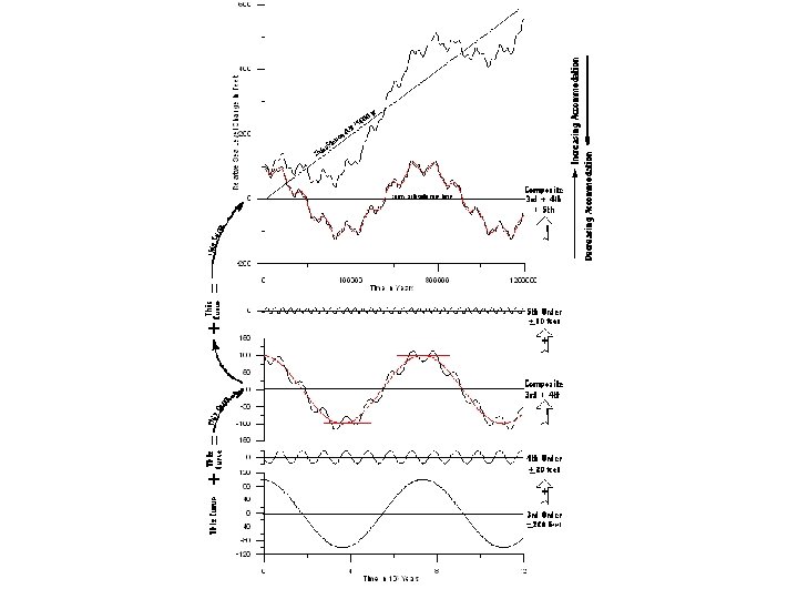
Universality Properties of Complex Evolutionary Systems Fractal Organization – Sea Level Changes 53

Universality Properties of Complex Evolutionary Systems Fractal Organization – Sea Level Changes patterns, within patterns 53

Graph to left takes up Only this much time on the Above graph Relative Sea Level Curves

Relative Sea Level Curves and Constructive and Destructive Interference 3 rd order down, 4 th order up; muted sea level fall 3 rd order up, 4 th order down; muted sea level rise Both curves go down; exaggerated sea level fall

Sea Level Changes and Corresponding Trangressions/Regressions are Fractal Third Order Transgression. . . followed by. . . A Third Order Regression

Sea Level Changes and Corresponding Trangressions/Regressions are Fractal Third Order Transgression. . . followed by. . . A Third Order Regression 4 th Order Regression. . . followed by. . . 4 th Transgression. . . followed by. . . 4 th Regression. . . followed by. . . 4 th Transgression followed by. . . 4 th Regression

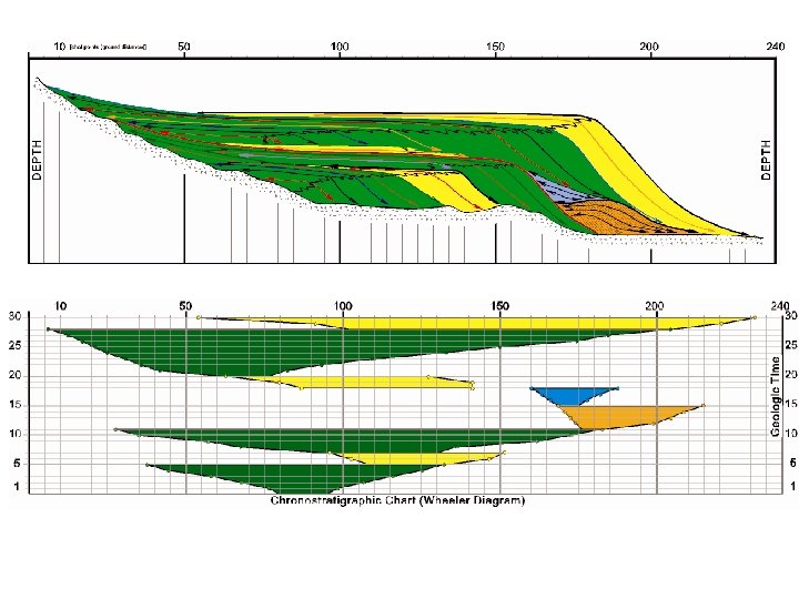
Sea Level Changes and Corresponding Trangressions/Regressions are Fractal FUS CUS Figure 8 shows upward and seaward increase in depositional energy (yellow dotted and green areas), which is tied to increases in porosity and permeability. The basal disconformity (wavy line) is the horizontal datum for the 3 -D porosity and permeability models. The wedge shape of the Sussex "B" interval results from reworking by currents of seaward margins of sand ridges, and landward redeposition of sediment. The blue-lined areas are basal and landward low-depositional-energy facies; these exhibit low porosity, permeability, and petroleum production. The disconformity at the top of the Sussex "B" sandstone is generally marked by a thin chert-pebble sandstone (figure 9 A). Shading variation of the quartz (figure 9 B) results from fracturing of the grain in this cross-nicols photomicrograph view (light is transmitted differently due to rotation of the crystal axes). Quartz grains that were incorporated from underlying sand-ridge sediments commonly exhibit early stages of diagenesis within marine environments, primarily chamosite overgrowths under the quartz overgrowths. Grain-to-grain contacts within this facies are mainly point with lesser long-straight contacts. http: //pubs. usgs. gov/dds-033/USGS_3 D/ssx_txt/depomod. htm

Correlation Demonstrating the Equivalency of Stratigraphic Units

Equivalency may mean: Lithologic: Paleontologic: Time: Same rock unit Contain same fossils Deposited at same time Biostratigraphic Facies # 2 Facies are the many different sediments and resulting rocks that form at the same time, but in different depositional environments. Facies # 1 Facies are the many different sediments and resulting rocks that form at the same time, but in different depositional environments.

1. Ways of Correlating - Lithologic “Walking Out” Physically tracing a bed from one place to another to insure it is in fact the same rock unit; literally “walking it out. ” Or, tracing an outcrop down the highway. Can be done in many places in the west where good exposure, and flat lying beds are easy to trace.

Grand Canyon of Arizona http: //www. mongabay. com/external/grand_canyon_trouble. htm http: //www. ggl. ulaval. ca/personnel/bourque/s 4/cambrien. pangee. html http: //www. raphaelk. co. uk/main/worldwonders. htm

http: //www. jgk. org/maps/grand-canyon-large. html

The problem is, . . . Rocks are not always flat laying, and traceable at the surface. A cross section through the Harrisonburg and Bridgewater, Virginia area, showing a duplex “herd of horses. ” The floor thrust is at the bottom of the drawing just above the basement rocks. The North Mountain fault is the roof thrust. In between are a series of splay faults that isolate a series of horses. Note the overturned anticline on the far left (west) side where the last ramp formed. From Gathright and Frischmann, 1986, Geology of the Harrisonburg and Bridgewater Quadrangles, Virginia.

2. Ways of Correlating - Lithologic “Key Beds” Correlating by recognizing and identifying beds that are so distinctive you always know them when you see them. 1. Distinctive lithology 2. Distinctive mineral assemblage. 3. Particular sedimentary structures.

“Key Beds” The Chattanooga Shale http: //www. uta. edu/paleomap/homepage/Schieberweb/summer_2000_field_work. htm

“Key Beds” The iridium layer at the KT boundary An analysis of the chemical composition of this clay layer shows that it contains a relatively high concentration of an element called iridium. Iridium is rare in the Earth’s crust, but more common towards the Earth's centre, and in space. It continually filters down to earth from outer space, and so a high concentration of iridium is usually an indication that the sediment was deposited very slowly, absorbing lots of iridium over time. http: //www. bbc. co. uk/beasts/whatkilled/evidence/analyse 1. shtml http: //c 3 po. barnesos. net/homepage/lpl/fieldtrips/K-T/day 3. html

http: //www. athro. com/geo/trp/ktmain. html The hill in the background of this photograph is known as Iridium Hill. The bands on the side of the hill are layers of rock of different ages that span the time of the extinction of the dinosaurs. http: //www. uhaul. com/supergraphics/crater/what-is-it 2. html http: //www. student. oulu. fi/~jkorteni/space/boundary /

“Key Beds” The Navajo Sandstone http: //www. mines. utah. edu/geo/about_ES/Geology/Zion. GIFS/Xbed. SS. html http: //www. olympic. ctc. edu/class/dassail/Cap. Reef. html http: //www. creationsafaris. com/crev 07. htm

3. Ways of Correlating - Lithologic “Position in Sequence” Identifying a relatively nondescript formation, which could be confused with other similar looking beds, by its relationship to other more distinctive units. Limestone Cross Bedded Sandstone Non-Descript Shale Quartz Arenite Arkose

4. Ways of Correlating - Lithologic “Wire Line Well Logging” Measuring geophysical properties of a rock as recorded by instruments lowered down a well hole. In logging the well four main types of equipment are used: the downhole instrument (which measures the data), the computerized surface data acquisition system (to store and analyze the data), the cable or wireline (which serves as both mechanical and data communication link with the downhole instruments), and the hoisting equipment to raise and lower the instruments. Resistivity Logs Gamma Ray Logs Acoustic Logs http: //www. bakerhughes. com/bakeratlas/about/log 4. htm

“Wire Line Well Logging” http: //www. trianaenergy. com/ucwell/photos/march_26. htm

Geophysical logging involves lowering a series of probes into drilled boreholes (or existing fractures or wells) as deep as several thousands of feet into the ground. One type of multiparameter probe that has been used in Maryland Delaware measures several characteristics of subsurface properties, including natural gamma radiation, or a material’s resistance to electric current, which is useful for finding a good water-bearing sand aquifer for water-supply purposes. Another type is an acoustic velocity probe, which works by transmitting acoustic signals and recording the traveltime of the acoustic wave from one or more transmitters to receivers in the probe. The recorded information can be used to measure porosity and calculate the material’s density. This technique was used to determine the extent of jumbled geologic strata caused by a crater impact at the mouth of the Chesapeake Bay 30 million years ago. Another type of probe, called an Acoustic Televiewer, transmits acoustic signals to subsurface rock layers and uses state-of-the-art computer software to convert the recorded data into an actual image of the borehole. This image can be used to determine the amount of water that could be extracted from individual fractures in the rock formation. Even though most of the parameters measured by these probes can only be determined in a newly drilled “open” borehole, certain probes emit signals that can penetrate well casings, making it possible to measure subsurface materials after a well is constructed. Gamma rays can travel through almost any type of well casing, while an “induction” probe can measure conductivity electromagnetically through polyvinyl chloride (PVC) casing. Other parameters, such as the borehole’s fluid temperature and conductivity, can also be measured, making it possible to evaluate water quality. The flow direction of ground water can also be determined with several types of probes. All of this equipment enables scientists to characterize the properties of subsurface materials, improving our knowledge of what lies beneath the Earth’s surface. http: //md. water. usgs. gov/publications/fs-126 -03/html/

A typical well logging arrangement and the resultant logs from two types of tools, the GR and Resistivity Logs http: //www. brookes. ac. uk/geology/8345 welc. html#Wireline

Gamma Ray Logs One of the advantages of gamma ray logs is that the gamma ray intensity closely corresponds with texture of the rocks. Typically, gamma ray radiation is higher with shales (because they have radioactive K 40 in them which undergoes K to Ar decay. ) Sandstones tend to have a lower gamma radiation. Thus, we can use the gamma ray log as a proxy for texture of the sediment, and this allows us to read them like a strip log, obtaining information about the energy of deposition. http: //www. kgs. ukans. edu/Dakota/vol 3/fy 89/app_b. htm

Gamma Ray Logs and Strip Logs Low Radioactivity SANDSTONE High Radioactivity SHALE Very rapid FUS Gamma Ray Trace from Well log Rapid FUS is a rapid rise in sea level. They are parasequence boundaries used for correlation. Converted into a Stratigraphic Strip log Coarsening Upward Sequence Observe that gamma ray strip logs are the mirror image of a regular strip log where texture increases to the right.

Gamma Ray Strip Logs Vary with Depositional Environment Shoreface Rapid FUS is a parasequence boundary used for correlation. Tidal Shoreline Subtler FUS is a parasequence boundary used for correlation. Rapid CUS is a parasequence boundary used for correlation.

Gamma Ray Correlation Followed by Facies Correlation Overall CUS Coastal Plain Shoreface Offshore Shelf Sea level rises affect large parts of the depositional basin, and their effects are therefore widespread making them ideal for correlations.

5. Ways of Correlating - Lithologic “Reflection Seismicity” Seismic surveys use low frequency acoustical energy generated by explosives or mechanical means. These waves travel downward, and as they cross the boundaries between rock layers, energy is reflected back to the surface and detected by sensors called geophones. The resulting data, combined with assumptions about the velocity of the waves through the rocks and the density of the rocks, are interpreted to generate maps of the formations. Seismic surveys are usually performed using multiple geophones set at known distances from the energy source. Early seismic surveys used mechanical plotters to record the received signals, and were restricted to a few geophones. These surveys placed the source and geophones in a straight line, with the interpretation of the resulting data producing a 2 -D cross section of the formation under that line. The interpretations were subject to error, which increased the difficulty, and cost, of accurately locating hydrocarbon-bearing formations. Today, the development of digital recording systems allow the recording of data from more that 10, 000 geophones simultaneously, greatly speeding data collection. Sophisticated computer programs develop highly accurate 3 -D models of rock structures. These models are more accurate than past 2 -D maps, and increase the likelihood of accurately identifying hydrocarbon-bearing formations. http: //www. bakerhughes. com/bakeratlas/about/log 2. htm

Dark lines are seismic reflection surfaces. Detailed study shows they are essentaily time lines corresponding also with lithologic contacts. http: //www. geocities. com/jtvanpopta/seismic_reflection. html

http: //www. bgr. de/b 322/index. html? /b 322/text/d_sunda. htm

Seismic profile across the Cocos and North American Plates adjacent to Costa Rica. Single and double-headed arrows delineate structural fabric in the crust and mantle http: //www. mala. bc. ca/~earles/hydrated-mantle-sep 03. htm

http: //www. gfz-potsdam. de/pb 4/pg 3/projects/3 -D_structural_modelling_CEBS/content_en. html

http: //www. niwa. cri. nz/pubs/wa/11 -3/images/news 4_large. jpg/view

Ways of Correlating – Biostratigraphic Correlation is based on the work of William Smith and George Cuviere who established the two principles by which geologic maps are drawn. 1. Principle of Faunal Succession The Subversive Fossil 2. Principle of Faunal Correlation It had been towards the end of the seventeenth century that the first very few and very bold observers raised (albeit timidly) the ultimate heretical thought: the possibility that perhaps, just perhaps, these objects actually were what collectors and scientists and countrymen had long been loath to consider admitting - the organic remains of the very creatures that they looked like. The same strata are always found in the same order of superposition, and they always contain the same peculiar fossils.

Basis of Biostratigrapic Correlation Zone: A body of rock characterized, recognized and identified by one or more of the fossils it contains. Range Zone: based on the entire vertical range of a single species. Assemblage Zone: based on the entire vertical range of a community of species. Teil Zone: “part zone” defined locally by only part of the known total range of a particular species. Peak Zone: based on the greatest abundance (the abundance peak) of a species.

Species 2 Species 12 Species 11 Species 10 Species 13 Species 9 Species 8 Species 7 Species 6 Species 5 Fossil 6 disappears Species 3 Species 4 Defining Biostratigraphic Zones Biostratigraphic Zone Based On Species 13 Biostratigraphic Zone Based On On Species 56 Fossil 6 first appears Assemblage Zone With Fossil 6

The Index Fossil Not all fossils are equally useful for correlation. Lingula, the inarticular brachiopod, for example appears in the record about 540 million years ago, and is still living today. The best knowledge we get from Lingula is that the rock was deposited between 450 million years ago and today. Not very useful. On the other hand, Lingula prefers to live in tidal systems and so does provide us with paleoenvironmental information.

The Index Fossil The fossils that are most useful for correlation possess the following characteristics: 1. Abundant – no one wants to spend hours looking for the index fossil. They should be easy to find. 2. Rapidly Evolving – want species that evolve and diversify rapidly so that small stratigraphic intervals can be distinguished. 3. Widely dispursed – the best index fossils are swimmers or floaters since their remains tend to show up in many different environments. Facies fossils, those living on the bottom in restricted habitats, are not as useful. There abundant practical problems associated with biostratigrapic correlation. Requires the work of specialists who have done the technical, nit-picking, careful, highly detailed work that is necessary.

The Relationship Between Lithologic and Biostratigraphic Correlation Local Section #1 Local Section #2 Biostratigraphic Correlation between local sections Fossil Zone n io at Time m o t ds n Sa ne n tio c e of r Fo gr ns a Tr n sio es r Di Lirthologic Correlation between local sections Hundreds of Miles

http: //www-odp. tamu. edu/publications/198_IR/chap_05/c 5_f 6. htm

http: //www-odp. tamu. edu/publications/183_SR/002/images/02_f 02. gif

Diastems and Unconformities Gaps in the Record Premise 1 – We want a complete history of the Earth. Premise 2 – The Record is preserved only in the rocks. Premise 3 – The Rock Record is incomplete, being destroyed by weathering and erosion, or lack of deposition. Therefore – A complete history of the Earth is not possible. Consequenctly, in order to understand the Earth’s history we must understand the gaps in the record, what is missing, why it is missing, and how we know.

Nonconformity Angular Disconformity

Angular Unconformity The Taconic Unconformity, an angular unconformity between the vertical beds of the Ordovician Austin Glen Formation and the overlying, but steeply dipping, Late Silurian Rondout Formation. http: //3 dparks. wr. usgs. gov/nyc/parks/loc 26. htm

Angular Unconformity http: //www. gly. uga. edu/railsback/Field. Images. htm

Angular Unconformity at Siccar Point James Hutton’s Famous Unconformity http: //www. gly. uga. edu/railsback/Field. Images. html

Angular Unconformity http: //geology. asu. edu/~sreynolds/glg 103/relative_age_principles. htm

Nonconformity http: //www. geowords. com/lostlinks/c 19/nonconformity. htm

Nonconformity Along U. S. Highway 67 south of Farmington, Missouri we came to a road cut which featured a very weathered section of granite (probably the Knob Lick granite) which is overlain by a sandstone layer (presumably the Lamotte). Shown in the image on the left, the granite layer is the white weathered debris on the bottom and the sandstone unit is the layered rock on top. http: //www. pittstate. edu/services/scied/Teachers/Field/Camp/Us 67 -1/us 67 -1. htm

Nonconformity View from Hout Bay towards Chapmans Peak, showing the nonconformity between the Cape Granite and strata of the Cape Supergroup. Cutting the granite and unconformity is a dolerite dyke http: //web. uct. ac. za/depts/geolsci/dlr/peninsula%20 geology. html

Disconformity Closer view of contact point between Lykins formation (reds) and Canyon Spring sandstone (whites). The greenish layer in between is where iron has leached out of the uppermost Lykins formation. A disconformity exists here because approx. 70 million years of deposition is missing here between the early Triassic Lykins formation and the mid-to-late Juarssic Canyon Spring sandstone. http: //www. paleocurrents. com/cert_classes/2003_03_15_5/HTML/img_8159. htm

Disconformity http: //www. gc. maricopa. edu/appliedscience/gjc-nsf/reldat 26. html http: //rockhounds. com/grand_hikes/cape_solitude/index. shtml

Diastems - 1 Invisible Gaps in the Record Erosion and Deposition on a Relative Sea Level Curve In this model a sea level rise leads to deposition, and a sea level fall to erosion and/or no deposition – resulting in a gap in the record. The model assumes a simple relationship: only sea level rises not countered by a drop result in a permanent record. A sea level rise with a corresponding drop at any time in the future results in no permanent record.

Diastems - 2 Nearly Invisible Gaps in the Record Condensed Section Parasequence Rapid Rise in Sea Level With sea level not changing much sediment fills in the accommodation resulting in a regression and a CUS Sea Level Rise Shoreline moves inland Shore Layer of black shale only a few mm or cm thick. Hard to see or find in ourcrop. Distal basin receives little sediment resulting in a condensed section Near Far Shelf Old Near Shelf now becomes deep, distal far shelf

Diastems - 2 Invisible Gaps in the Record Low Radioactivity SANDSTONE Condensed Sections in Parasequences A parasequence is a deposit laid down between two pulses of sea level rise. Condensed Section Is only mm to a cm thick But contains as much Time as the rest of The parasequence Rapid Rise in Sea Level Parasequence Slowing of rise in sea Level; deposition Catches up to increase In water depth High Radioactivity SHALE Condensed Section Rapid rise in sea level at this point puts the section distally away from the source land. Sediment can no longer reach it and only a very thin deposit is laid down, almost too thin to notice.

Diastems - 3 Invisible Gaps in the Record Episodic Depositional Events When we look at an outcrop of rock is it easy to think that it represents continuous deposition. After all, we don’t see any gaps or holes in the outcrop. Yet, there are lots of holes (gaps) and not all deposits represent equivalent time. Most of the beds we see in an outcrop represent geologically instantaneous events. They took at most a few hours or a few days to be deposited. The shale beds in between represent slow deposition over years of time. The outcrop is a kaleidoscope of different lengths of time – and they are fractal. Most of the record is in fact gap. We see the rocks, but we do not see the gaps. Low Radioactivity SANDSTONE High Radioactivity SHALE But, this shale may represent a year or years or decades of time. A few hours of time to deposit this.