Stochastic Optimization is almost as Easy as Deterministic

Stochastic Optimization is (almost) as Easy as Deterministic Optimization Chaitanya Swamy Caltech Joint work with David Shmoys done while at Cornell University

Stochastic Optimization • Way of modeling uncertainty. • Exact data is unavailable or expensive – data is uncertain, specified by a probability distribution. • Want to make the best decisions given this uncertainty in the data. Applications in logistics, transportation models, financial instruments, network design, production planning, … • Dates back to 1950’s and the work of Dantzig.

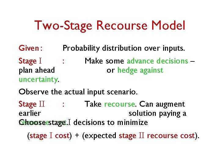
Two-Stage Recourse Model Given : Probability distribution over inputs. Stage I : Make some advance decisions – plan ahead or hedge against uncertainty. Observe the actual input scenario. Stage II : Take recourse. Can augment earlier solution paying a Choose recoursestage cost. I decisions to minimize (stage I cost) + (expected stage II recourse cost).

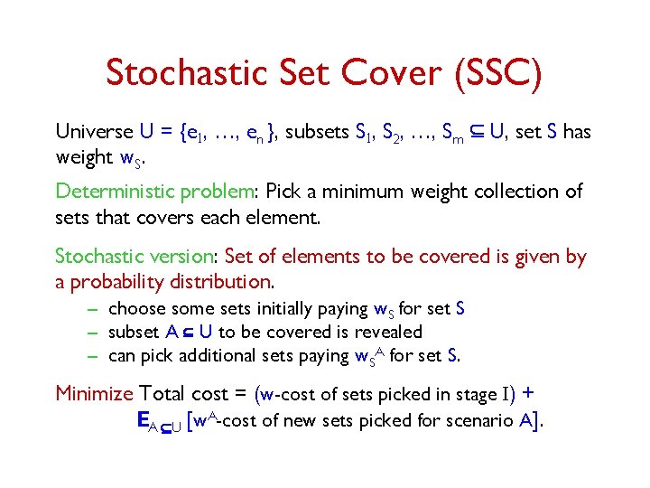
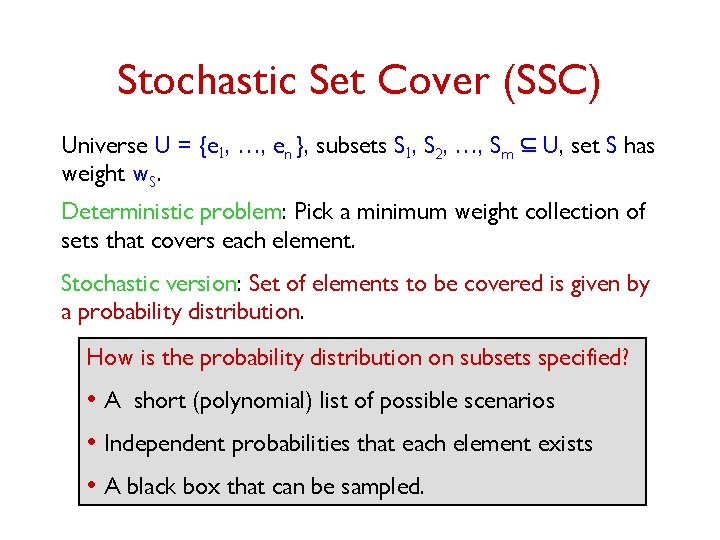
Stochastic Set Cover (SSC) Universe U = {e 1, …, en }, subsets S 1, S 2, …, Sm Í U, set S has weight w. S. Deterministic problem: Pick a minimum weight collection of sets that covers each element. Stochastic version: Set of elements to be covered is given by a probability distribution. – choose some sets initially paying w. S for set S – subset A Í U to be covered is revealed – can pick additional sets paying w. SA for set S. Minimize Total cost = (w-cost of sets picked in stage I) + EA ÍU [w. A-cost of new sets picked for scenario A].

Stochastic Set Cover (SSC) Universe U = {e 1, …, en }, subsets S 1, S 2, …, Sm Í U, set S has weight w. S. Deterministic problem: Pick a minimum weight collection of sets that covers each element. Stochastic version: Set of elements to be covered is given by a probability distribution. How is the probability distribution on subsets specified? • A short (polynomial) list of possible scenarios • Independent probabilities that each element exists • A black box that can be sampled.

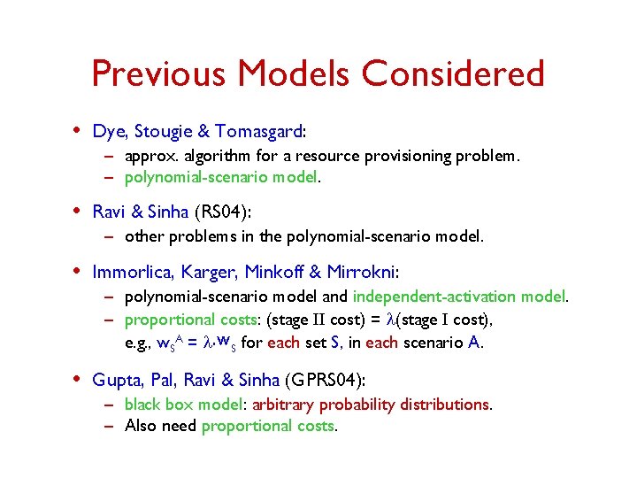
Previous Models Considered • Dye, Stougie & Tomasgard: – approx. algorithm for a resource provisioning problem. – polynomial-scenario model. • Ravi & Sinha (RS 04): – other problems in the polynomial-scenario model. • Immorlica, Karger, Minkoff & Mirrokni: – polynomial-scenario model and independent-activation model. – proportional costs: (stage II cost) = l(stage I cost), e. g. , w. SA = l. w. S for each set S, in each scenario A. • Gupta, Pal, Ravi & Sinha (GPRS 04): – black box model: arbitrary probability distributions. – Also need proportional costs.

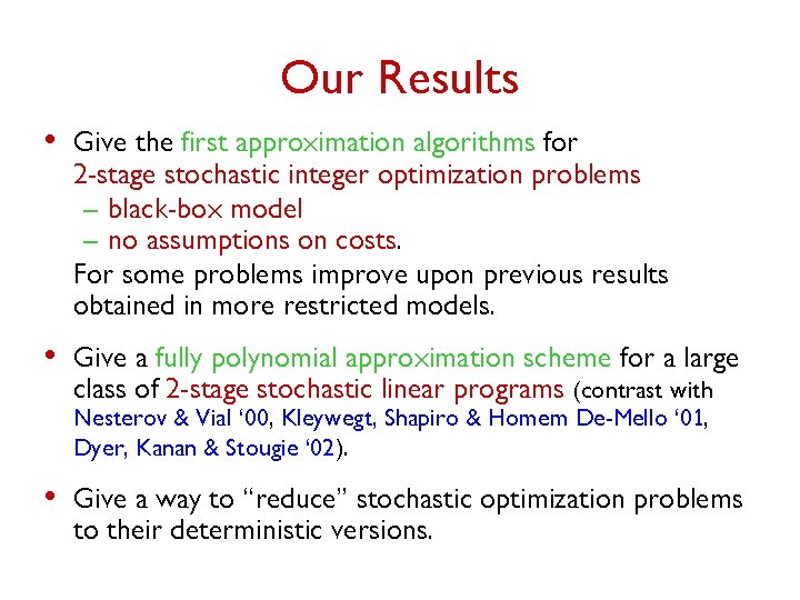
Our Results • Give the first approximation algorithms for 2 -stage stochastic integer optimization problems – black-box model – no assumptions on costs. For some problems improve upon previous results obtained in more restricted models. • Give a fully polynomial approximation scheme for a large class of 2 -stage stochastic linear programs (contrast with Nesterov & Vial ‘ 00, Kleywegt, Shapiro & Homem De-Mello ‘ 01, Dyer, Kanan & Stougie ‘ 02). • Give a way to “reduce” stochastic optimization problems to their deterministic versions.

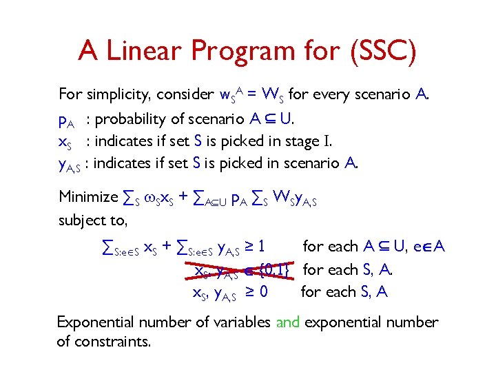
A Linear An Integer. Programfor for(SSC) For simplicity, consider w. SA = WS for every scenario A. p. A : probability of scenario A Í U. x. S : indicates if set S is picked in stage I. y. A, S : indicates if set S is picked in scenario A. Minimize ∑S w. Sx. S + ∑AÍU p. A ∑S WSy. A, S subject to, ∑S: eÎS x. S + ∑S: eÎS y. A, S ≥ 1 for each A Í U, eÎA x. S, y. A, S Î {0, 1} for each S, A. x. S, y. A, S ≥ 0 for each S, A Exponential number of variables and exponential number of constraints.

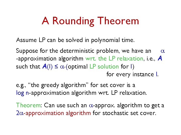
A Rounding Theorem Assume LP can be solved in polynomial time. Suppose for the deterministic problem, we have an a -approximation algorithm wrt. the LP relaxation, i. e. , A such that A(I) ≤ a. (optimal LP solution for I) for every instance I. e. g. , “the greedy algorithm” for set cover is a log n-approximation algorithm wrt. LP relaxation. Theorem: Can use such an a-approx. algorithm to get a 2 a-approximation algorithm for stochastic set cover.

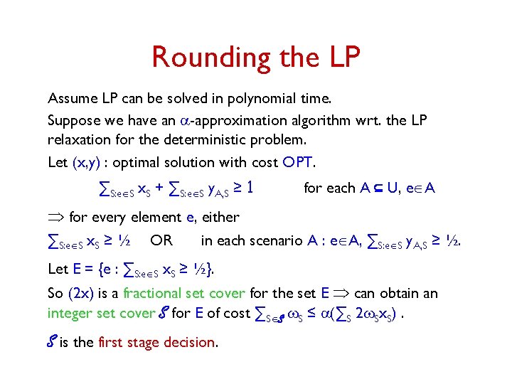
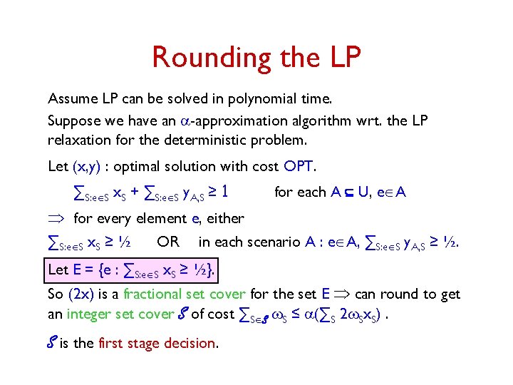
Rounding the LP Assume LP can be solved in polynomial time. Suppose we have an a-approximation algorithm wrt. the LP relaxation for the deterministic problem. Let (x, y) : optimal solution with cost OPT. ∑S: eÎS x. S + ∑S: eÎS y. A, S ≥ 1 for each A Í U, eÎA Þ for every element e, either ∑S: eÎS x. S ≥ ½ OR in each scenario A : eÎA, ∑S: eÎS y. A, S ≥ ½. Let E = {e : ∑S: eÎS x. S ≥ ½}. So (2 x) is a fractional set cover for the set E Þ can obtain an integer set cover S for E of cost ∑SÎS w. S ≤ a(∑S 2 w. Sx. S). S is the first stage decision.

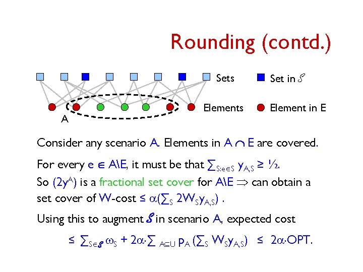
Rounding (contd. ) Sets Elements A Set in S Element in E Consider any scenario A. Elements in A Ç E are covered. For every e Î AE, it must be that ∑S: eÎS y. A, S ≥ ½. So (2 y. A) is a fractional set cover for AE Þ can obtain a set cover of W-cost ≤ a(∑S 2 WSy. A, S). Using this to augment S in scenario A, expected cost ≤ ∑SÎS w. S + 2 a. ∑ AÍU p. A (∑S WSy. A, S) ≤ 2 a. OPT.

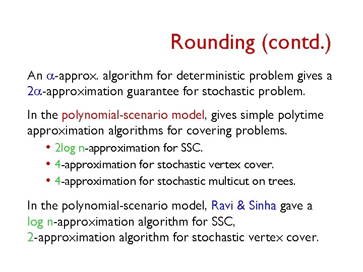
Rounding (contd. ) An a-approx. algorithm for deterministic problem gives a 2 a-approximation guarantee for stochastic problem. In the polynomial-scenario model, gives simple polytime approximation algorithms for covering problems. • 2 log n-approximation for SSC. • 4 -approximation for stochastic vertex cover. • 4 -approximation for stochastic multicut on trees. In the polynomial-scenario model, Ravi & Sinha gave a log n-approximation algorithm for SSC, 2 -approximation algorithm for stochastic vertex cover.

Rounding the LP Assume LP can be solved in polynomial time. Suppose we have an a-approximation algorithm wrt. the LP relaxation for the deterministic problem. Let (x, y) : optimal solution with cost OPT. ∑S: eÎS x. S + ∑S: eÎS y. A, S ≥ 1 for each A Í U, eÎA Þ for every element e, either ∑S: eÎS x. S ≥ ½ OR in each scenario A : eÎA, ∑S: eÎS y. A, S ≥ ½. Let E = {e : ∑S: eÎS x. S ≥ ½}. So (2 x) is a fractional set cover for the set E Þ can round to get an integer set cover S of cost ∑SÎS w. S ≤ a(∑S 2 w. Sx. S). S is the first stage decision.

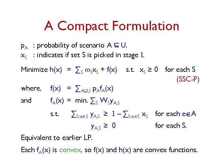
A Compact Formulation p. A : probability of scenario A Í U. x. S : indicates if set S is picked in stage I. Minimize h(x) = ∑S w. Sx. S + f(x) where, f(x) = ∑AÍU p. Af. A(x) and f. A(x) = min. ∑S WSy. A, S s. t. x. S ≥ 0 for each S (SSC-P) ∑S: eÎS y. A, S ≥ 1 – ∑S: eÎS x. S for each eÎA y. A, S ≥ 0 for each S. Equivalent to earlier LP. Each f. A(x) is convex, so f(x) and h(x) are convex functions.

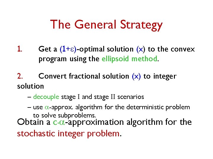
The General Strategy 1. Get a (1+e)-optimal solution (x) to the convex program using the ellipsoid method. 2. Convert fractional solution (x) to integer solution – decouple stage I and stage II scenarios – use a-approx. algorithm for the deterministic problem to solve subproblems. Obtain a c. a-approximation algorithm for the stochastic integer problem.

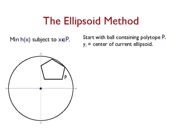
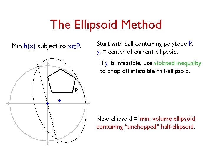
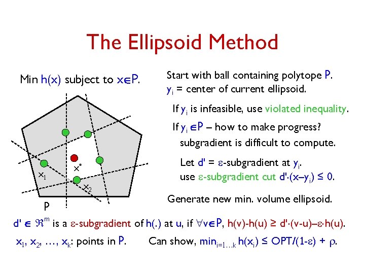
The Ellipsoid Method Min h(x) subject to xÎP. P Start with ball containing polytope P. yi = center of current ellipsoid.

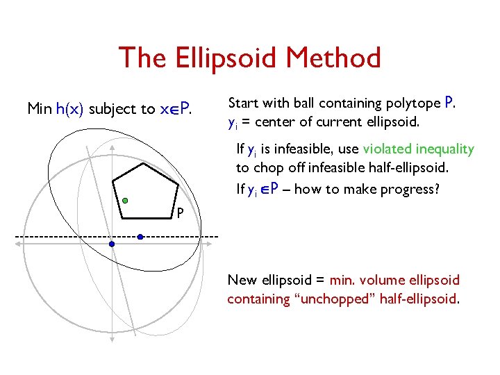
The Ellipsoid Method Min h(x) subject to xÎP. Start with ball containing polytope P. yi = center of current ellipsoid. If yi is infeasible, use violated inequality to chop off infeasible half-ellipsoid. P New ellipsoid = min. volume ellipsoid containing “unchopped” half-ellipsoid.

The Ellipsoid Method Min h(x) subject to xÎP. Start with ball containing polytope P. yi = center of current ellipsoid. If yi is infeasible, use violated inequality to chop off infeasible half-ellipsoid. If yi ÎP – how to make progress? P New ellipsoid = min. volume ellipsoid containing “unchopped” half-ellipsoid.

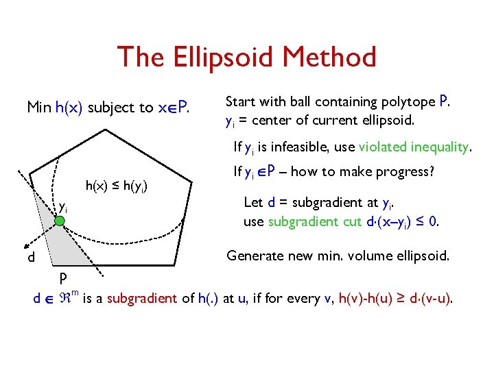
The Ellipsoid Method Min h(x) subject to xÎP. Start with ball containing polytope P. yi = center of current ellipsoid. If yi is infeasible, use violated inequality. h(x) ≤ h(yi) yi d If yi ÎP – how to make progress? Let d = subgradient at yi. use subgradient cut d. (x–yi) ≤ 0. Generate new min. volume ellipsoid. P d Î m is a subgradient of h(. ) at u, if for every v, h(v)-h(u) ≥ d. (v-u).

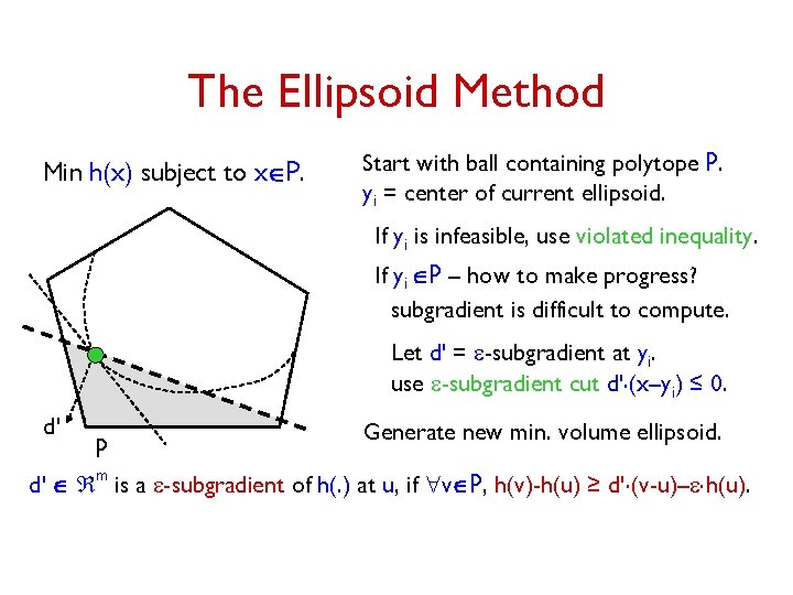
The Ellipsoid Method Min h(x) subject to xÎP. Start with ball containing polytope P. yi = center of current ellipsoid. If yi is infeasible, use violated inequality. If yi ÎP – how to make progress? subgradient is difficult to compute. Let d' = e-subgradient at yi. use e-subgradient cut d'. (x–yi) ≤ 0. d' P Generate new min. volume ellipsoid. d' Î m is a e-subgradient of h(. ) at u, if "vÎP, h(v)-h(u) ≥ d'. (v-u)–e. h(u).

The Ellipsoid Method Min h(x) subject to xÎP. Start with ball containing polytope P. yi = center of current ellipsoid. If yi is infeasible, use violated inequality. If yi ÎP – how to make progress? subgradient is difficult to compute. x 1 x* x 2 P Let d' = e-subgradient at yi. use e-subgradient cut d'. (x–yi) ≤ 0. Generate new min. volume ellipsoid. d' Î m is a e-subgradient of h(. ) at u, if "vÎP, h(v)-h(u) ≥ d'. (v-u)–e. h(u). x 1, x 2, …, xk: points in P. Can show, mini=1…k h(xi) ≤ OPT/(1 -e) + r.

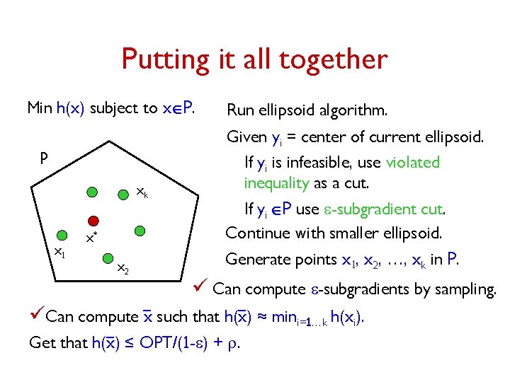
Putting it all together Min h(x) subject to xÎP. Run ellipsoid algorithm. Given yi = center of current ellipsoid. P xk x 1 x* x 2 If yi is infeasible, use violated inequality as a cut. If yi ÎP use e-subgradient cut. Continue with smaller ellipsoid. Generate points x 1, x 2, …, xk in P. ü Can compute e-subgradients by sampling. üCan compute x such that h(x) ≈ mini=1…k h(xi). Get that h(x) ≤ OPT/(1 -e) + r.

Sample Average Approximation (SAA) method: – Sample initially N times from scenario distribution – Solve 2 -stage problem estimating p. A with frequency of occurrence of scenario A How large should N be? Kleywegt, Shapiro & Homem De-Mello (KSH 01): – bound N by variance of a certain quantity – need not be polynomially bounded even for our class of programs. Recently, Charikar & Chekuri, Shmoys & S: – show that for a large class of stochastic LPs, N can be poly-bounded. Nemirovskii & Shapiro: – show that for SSC with non-scenario dependent costs, KSH 01 gives polynomial bound on N for (preprocessing + SAA) algorithm.

Summary of Results • Give an approximation scheme to solve a broad class of stochastic linear programs. • Obtain the first approximation algorithms for 2 -stage stochastic integer problems – no assumptions on costs or probability distribution. – 2 log n-approx. for set cover – 4 -approx. for vertex cover and multicut on trees. – 3. 23 -approx. for uncapacitated facility location (FL). Get constant guarantees for several variants such as FL with penalties, or soft capacities, or services. – (1+e)-approx. for multicommodity flow. Generalize and/or improve results of GPRS 04, Immorlica et al. obtained in restricted models. • Give a general technique to lift deterministic guarantees to stochastic setting.

Open Questions • Practical Impact: Can one use e-subgradients in other deterministic optimization methods, e. g. , cutting plane methods? Interior-point algorithms? • Multi-stage stochastic optimization. • Characterize which deterministic problems are “easy to solve” in stochastic setting, and which problems are “hard”.

Thank You.