Stochastic Inventory Modeling Chapter 16 Assumptions in Deterministic

Stochastic Inventory Modeling Chapter 16

Assumptions in Deterministic Models 1. 2. 3. 4. Demand is known and constant Lead time is known and constant Order quantity does not depend on price Order quantity arrives all at once when needed 5. Planned shortages are not allowed – Relaxed the 3 rd, 4 th and 5 th assumption

Independent Demand • Inventory exists to meet the demand of customers. • Customers can be external (purchasers of products) or internal (workers using material). • Management needs accurate forecast of demand. • Items that are used internally to produce a final product are referred to as dependent demand items. • Items that are final products demanded by an external customer are independent demand items.

Deterministic and Stochastic Models • If demand lead time are known (constant), they are called deterministic models • If they are treated as random (unknown), they are stochastic • Each random variable can have a probability distribution • Attention is focused on the distribution of demand during the lead time

Inventory Control Systems • Three basic types of systems: • continuous model (fixed-order quantity), periodic model (fixed-time), and Single-Period model • Continuous system: an order is placed for the same constant amount when inventory decreases to a specified level. • Periodic system: an order is placed for a variable amount after a specified period of time. • Single-period system: an order is placed just for one period

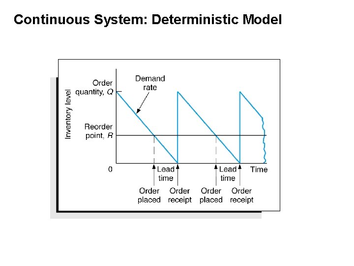
Continuous Inventory Systems • Continual record of inventory level is maintained. • Whenever inventory decreases to a predetermined level, the reorder point, an order is placed for a fixed amount • Management must be aware of status of inventory level • System is relatively expensive to maintain

Continuous System: Deterministic Model

Reorder Point • The reorder point is the inventory level at which a new order is placed. • Order must be made while there is enough stock in place to cover demand during lead time. • Formulation: • R = d. L • where d = demand rate per time period • L = lead time

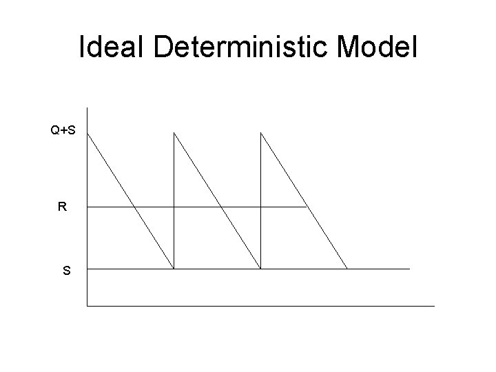
Ideal Deterministic Model Q+S R S

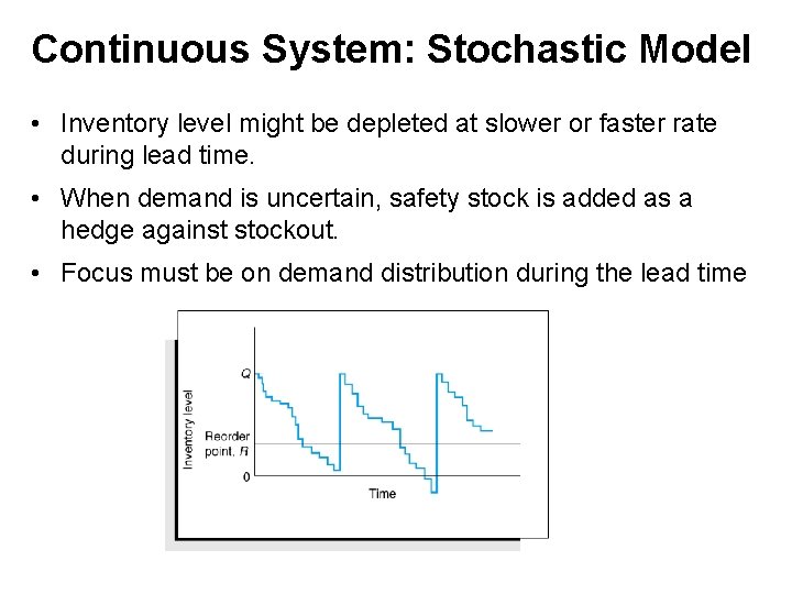
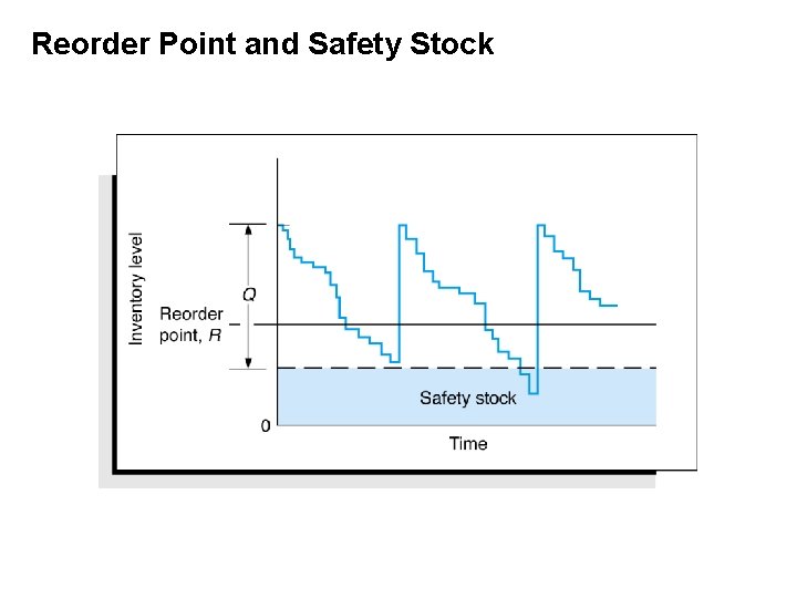
Continuous System: Stochastic Model • Inventory level might be depleted at slower or faster rate during lead time. • When demand is uncertain, safety stock is added as a hedge against stockout. • Focus must be on demand distribution during the lead time

Reorder Point and Safety Stock

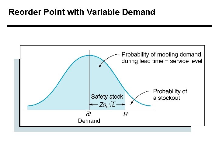
Reorder Point Quantity • Under deterministic conditions, when both demand lead time are constant, the reorder point is set equal to lead time demand. • Under probabilistic conditions, when demand and/or lead time varies, the reorder point often includes safety stock • Safety stock is the amount by which the reorder point exceeds the expected (average) lead time demand.

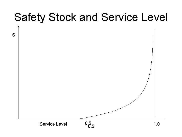
Safety Stock and Service Level • Safety stock determines the chance of a stockout during lead time • The complement of this chance is called the service level • Service level is defined as the probability of not incurring a stockout during any one lead time • The higher the probability inventory will be on hand, the more likely customer demand will be met. • Service level of 90% means there is a. 90 probability that demand will be met during lead time and. 10 probability of a stockout.

Safety Stock and Service Level S Service Level 0. 5 1. 0

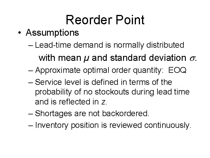
Reorder Point • Assumptions – Lead-time demand is normally distributed with mean µ and standard deviation . – Approximate optimal order quantity: EOQ – Service level is defined in terms of the probability of no stockouts during lead time and is reflected in z. – Shortages are not backordered. – Inventory position is reviewed continuously.

Reorder Point with Variable Demand

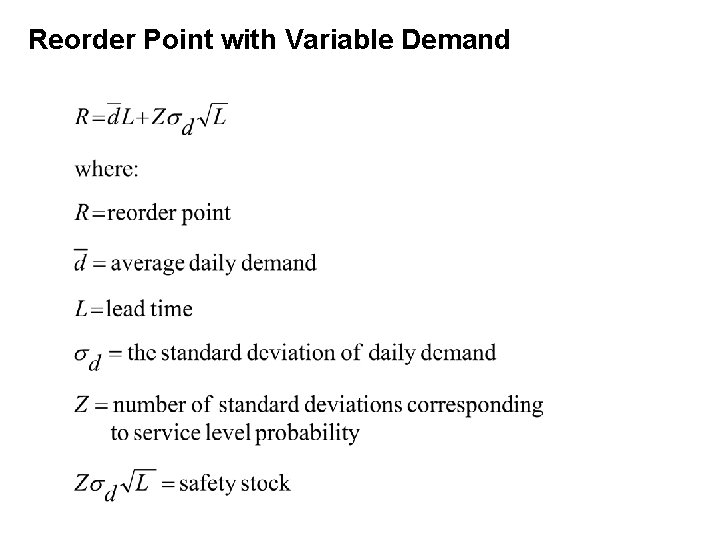
Reorder Point with Variable Demand

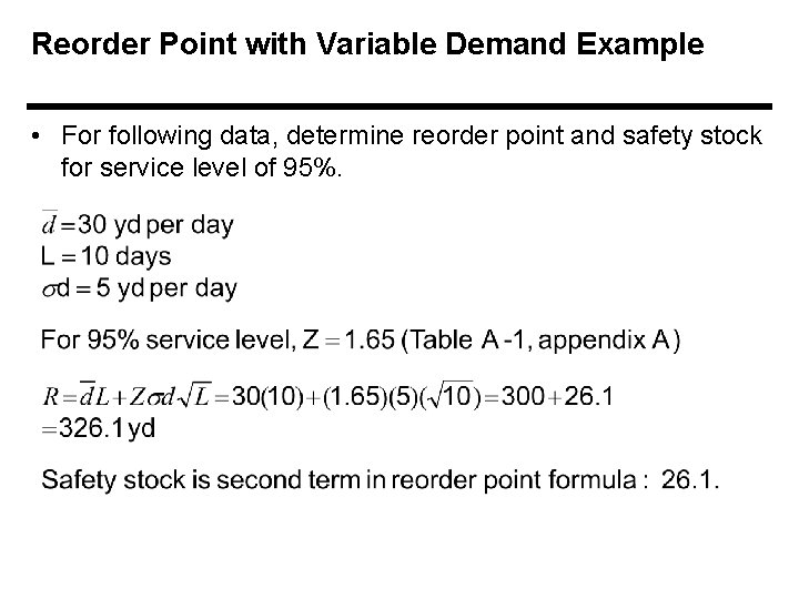
Reorder Point with Variable Demand Example • For following data, determine reorder point and safety stock for service level of 95%.

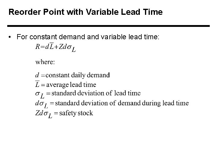
Reorder Point with Variable Lead Time • For constant demand variable lead time:

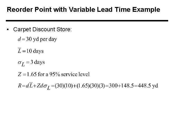
Reorder Point with Variable Lead Time Example • Carpet Discount Store:

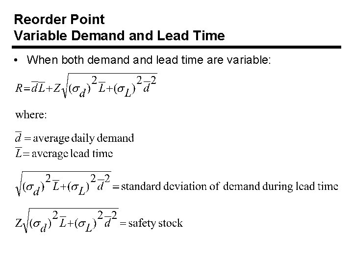
Reorder Point Variable Demand Lead Time • When both demand lead time are variable:

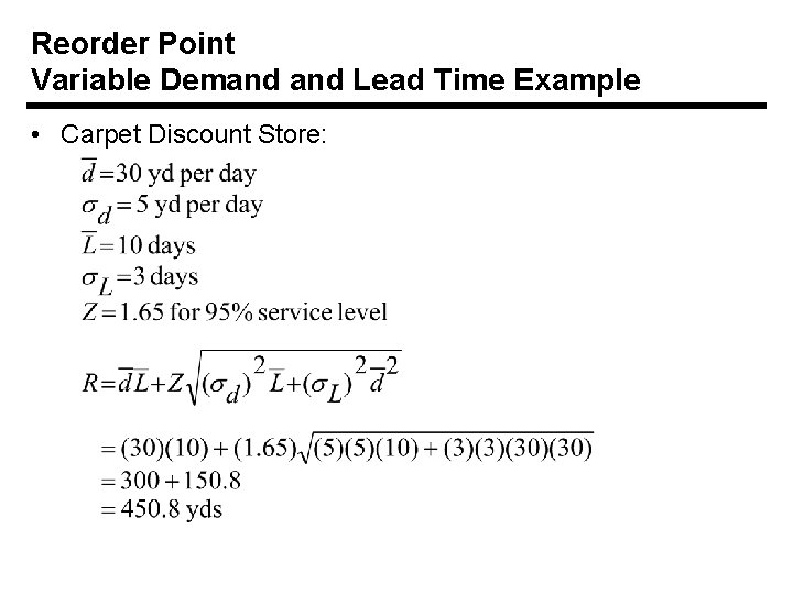
Reorder Point Variable Demand Lead Time Example • Carpet Discount Store:

Periodic Inventory Systems • Inventory level (on hand) is counted at specific time intervals • An order placed that brings inventory up to a specified level • Less costly to track of inventory level • Requires a new order quantity each time an order is placed • Used in smaller retail stores, drugstores, grocery stores and offices

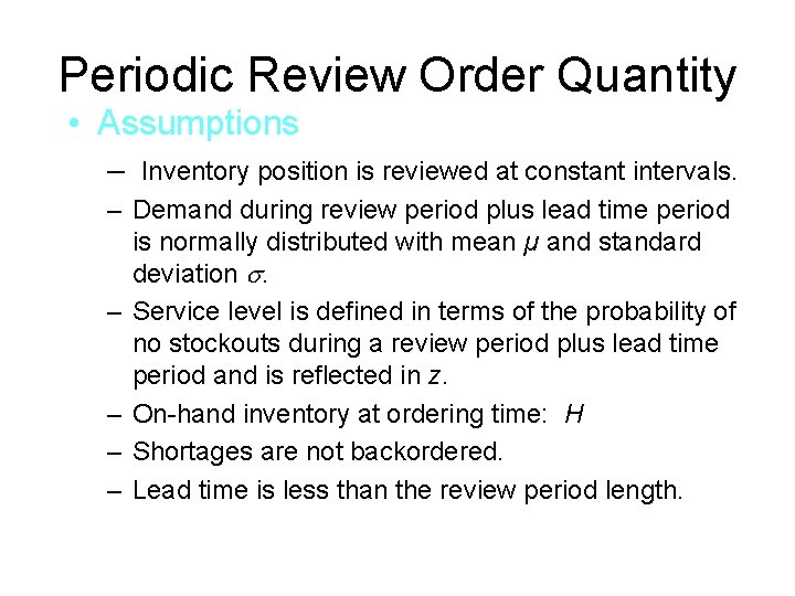
Periodic Review Order Quantity • Assumptions – Inventory position is reviewed at constant intervals. – Demand during review period plus lead time period is normally distributed with mean µ and standard deviation . – Service level is defined in terms of the probability of no stockouts during a review period plus lead time period and is reflected in z. – On-hand inventory at ordering time: H – Shortages are not backordered. – Lead time is less than the review period length.

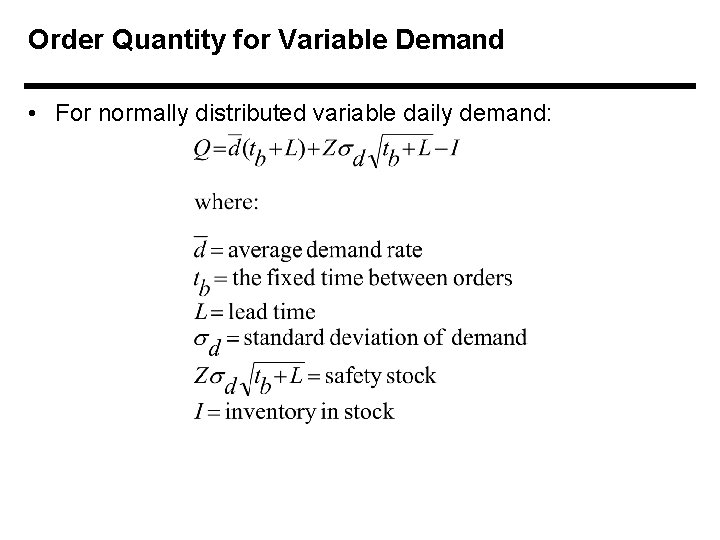
Order Quantity for Variable Demand • For normally distributed variable daily demand:

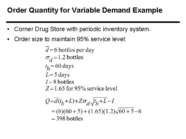
Order Quantity for Variable Demand Example • Corner Drug Store with periodic inventory system. • Order size to maintain 95% service level:

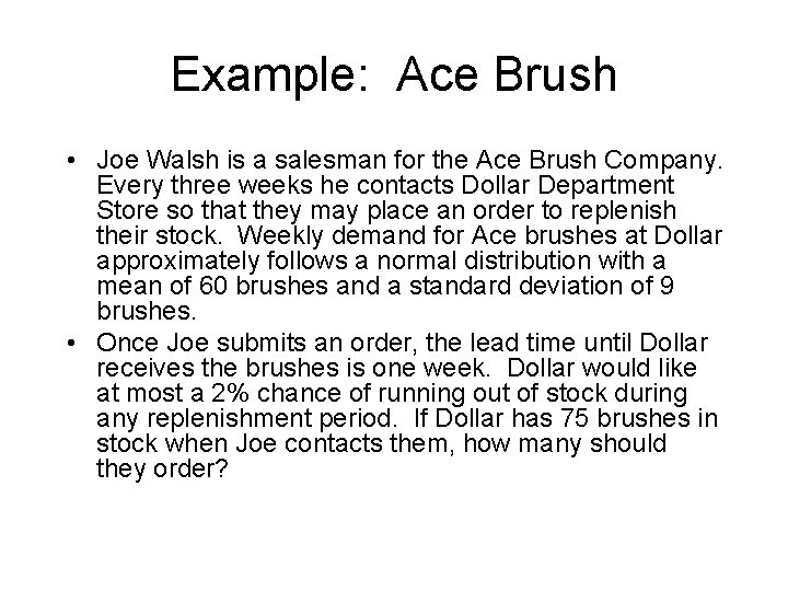
Example: Ace Brush • Joe Walsh is a salesman for the Ace Brush Company. Every three weeks he contacts Dollar Department Store so that they may place an order to replenish their stock. Weekly demand for Ace brushes at Dollar approximately follows a normal distribution with a mean of 60 brushes and a standard deviation of 9 brushes. • Once Joe submits an order, the lead time until Dollar receives the brushes is one week. Dollar would like at most a 2% chance of running out of stock during any replenishment period. If Dollar has 75 brushes in stock when Joe contacts them, how many should they order?

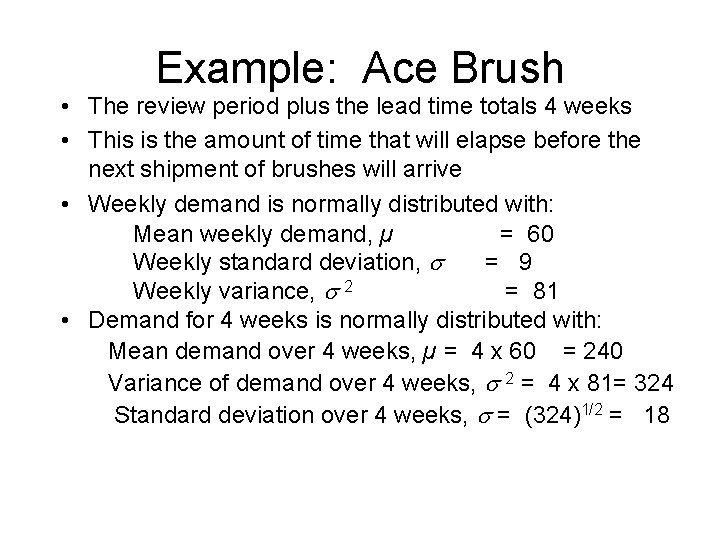
Example: Ace Brush • The review period plus the lead time totals 4 weeks • This is the amount of time that will elapse before the next shipment of brushes will arrive • Weekly demand is normally distributed with: Mean weekly demand, µ = 60 Weekly standard deviation, = 9 Weekly variance, 2 = 81 • Demand for 4 weeks is normally distributed with: Mean demand over 4 weeks, µ = 4 x 60 = 240 Variance of demand over 4 weeks, 2 = 4 x 81= 324 Standard deviation over 4 weeks, = (324)1/2 = 18

Single-Period Order Quantity • A single-period order quantity model (sometimes called the newsboy problem) deals with a situation in which only one order is placed for the item and the demand is probabilistic. • If the period's demand exceeds the order quantity, the demand is not backordered and revenue (profit) will be lost. • If demand is less than the order quantity, the surplus stock is sold at the end of the period (usually for less than the original purchase price).

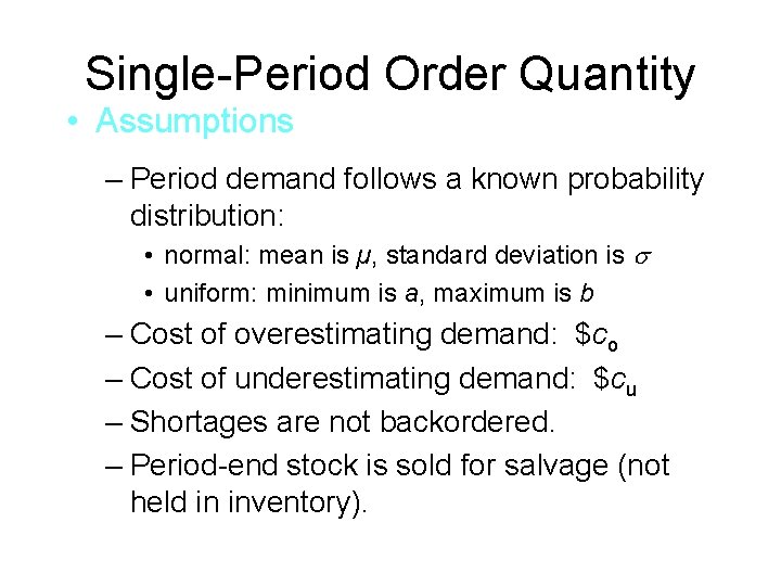
Single-Period Order Quantity • Assumptions – Period demand follows a known probability distribution: • normal: mean is µ, standard deviation is • uniform: minimum is a, maximum is b – Cost of overestimating demand: $co – Cost of underestimating demand: $cu – Shortages are not backordered. – Period-end stock is sold for salvage (not held in inventory).

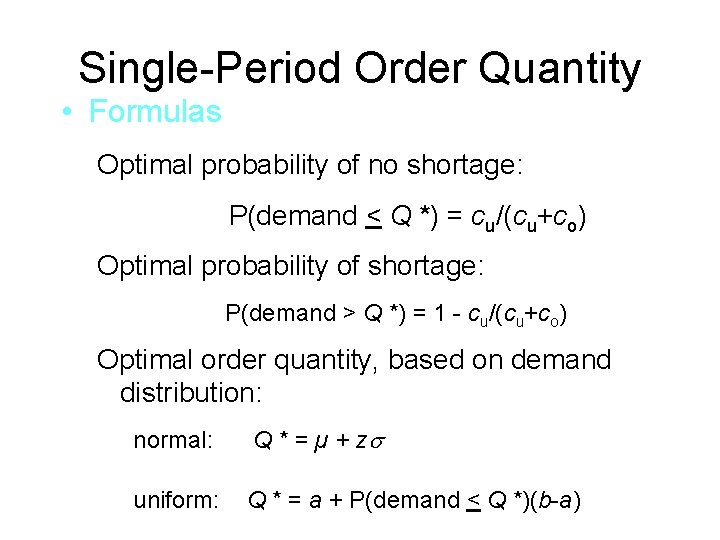
Single-Period Order Quantity • Formulas Optimal probability of no shortage: P(demand < Q *) = cu/(cu+co) Optimal probability of shortage: P(demand > Q *) = 1 - cu/(cu+co) Optimal order quantity, based on demand distribution: normal: Q * = µ + z uniform: Q * = a + P(demand < Q *)(b-a)

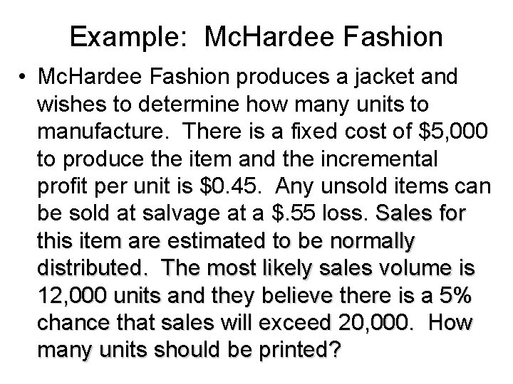
Example: Mc. Hardee Fashion • Mc. Hardee Fashion produces a jacket and wishes to determine how many units to manufacture. There is a fixed cost of $5, 000 to produce the item and the incremental profit per unit is $0. 45. Any unsold items can be sold at salvage at a $. 55 loss. Sales for this item are estimated to be normally distributed. The most likely sales volume is 12, 000 units and they believe there is a 5% chance that sales will exceed 20, 000. How many units should be printed?

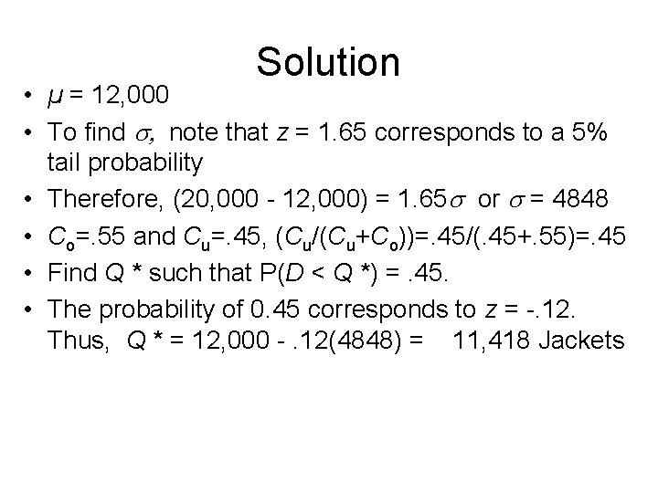
Solution • µ = 12, 000 • To find , note that z = 1. 65 corresponds to a 5% tail probability • Therefore, (20, 000 - 12, 000) = 1. 65 or = 4848 • Co=. 55 and Cu=. 45, (Cu/(Cu+Co))=. 45/(. 45+. 55)=. 45 • Find Q * such that P(D < Q *) =. 45. • The probability of 0. 45 corresponds to z = -. 12. Thus, Q * = 12, 000 -. 12(4848) = 11, 418 Jackets

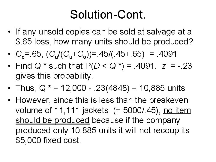
Solution-Cont. • If any unsold copies can be sold at salvage at a $. 65 loss, how many units should be produced? • Co=. 65, (Cu/(Cu+Co))=. 45/(. 45+. 65) =. 4091 • Find Q * such that P(D < Q *) =. 4091. z = -. 23 gives this probability. • Thus, Q * = 12, 000 -. 23(4848) = 10, 885 units • However, since this is less than the breakeven volume of 11, 111 jackets (= 5000/. 45), no item should be produced because if the company produced only 10, 885 units it will not recoup its $5, 000 fixed cost.