Steepest Descent Optimization Outline Regularized Newton Method Trust

Steepest Descent Optimization

Outline • • • Regularized Newton Method Trust Region Method for Line Search Solving Linear System of Equations Traveltime Tomography Conjugate Gradient Method

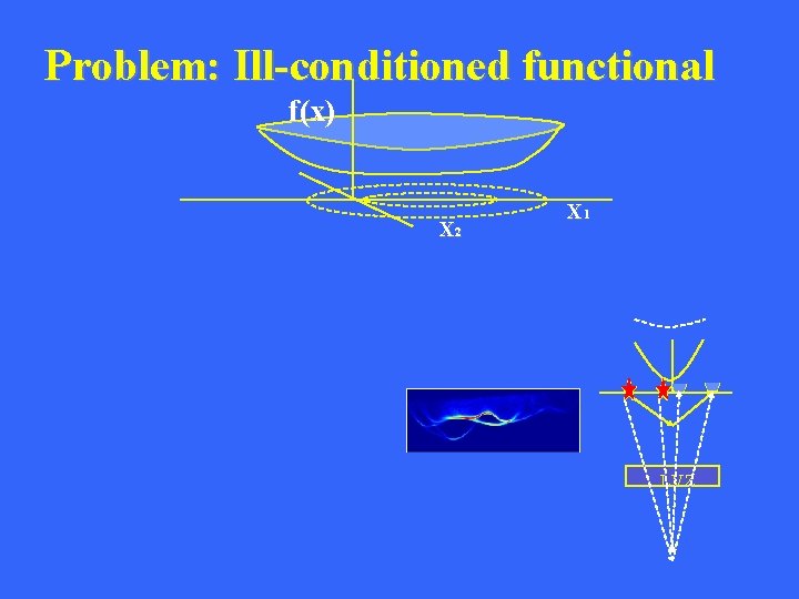
Problem: Ill-conditioned functional f(x) X 2 X 1 Examples: 1). Many models fit the same data 2). Seismic Data with short src-rec offset insensitive to deep part of model 3). Seismic Data from shallow loud vs soft from deep part of model 4). More unknowns than equations -> non-unique solution 5). Traveltime tomography LVZ

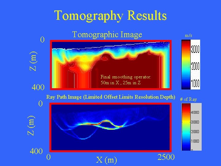
Tomography Results Tomographic Image Z (m) 0 m/s Final smoothing operator: 50 m in X , 25 m in Z 400 Z (m) 0 Ray Path Image (Limited Offset Limits Resolution Depth) # of Ray 400 0 X (m) 2500

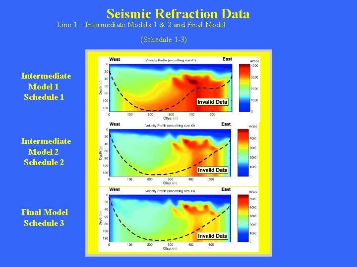
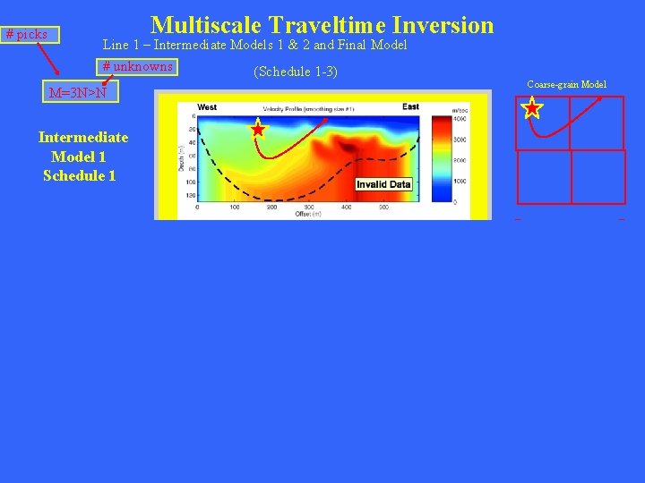
Seismic Refraction Data Line 1 – Intermediate Models 1 & 2 and Final Model (Schedule 1 -3) Intermediate Model 1 Schedule 1 Intermediate Model 2 Schedule 2 Final Model Schedule 3

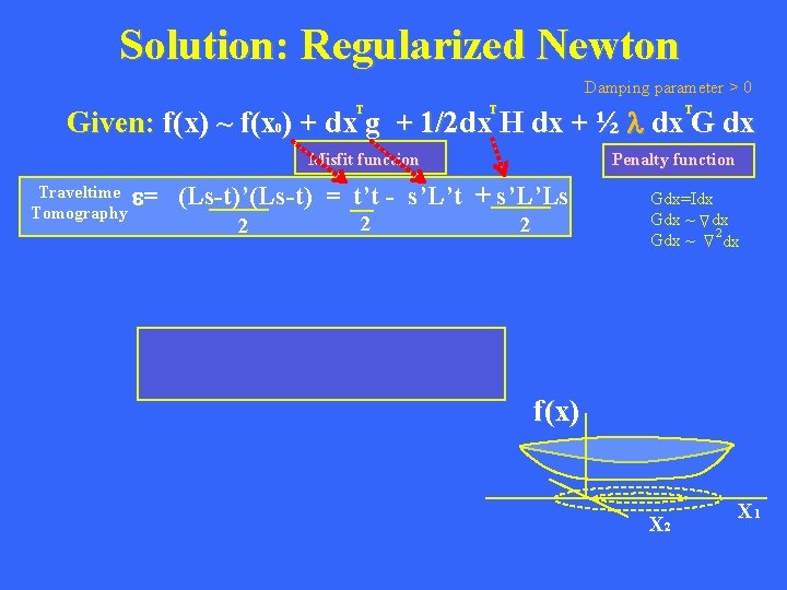
Solution: Regularized Newton Damping parameter > 0 Given: f(x) ~ f(x ) + dx g + 1/2 dx H dx + ½ l dx G dx T T T 0 (Ls-t)’(Ls-t) = t’t - s’L’t + s’L’Ls 2 2 Find: stationary point x* s. t. 2 D Traveltime e= Tomography Penalty function f(x*)=0 Gdx=Idx Gdx ~ dx 2 Gdx ~ dx D D Misfit function Soln: Newton’s Method (k) -1 x = x – a[H + l G] g (k+1) (k) f(x) . 02 max(H_ij) l Iteration number X 2 X 1

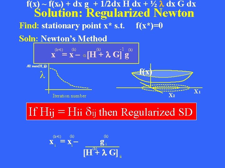
f(x) ~ f(x ) + dx g + 1/2 dx H dx + ½ l dx G dx 0 Solution: Regularized Newton Find: stationary point x* s. t. Soln: Newton’s Method (k+1) (k) -1 f(x*)=0 (k) x = x – a[H + l G] g. 02 max(H_ij) f(x) l Iteration number SD->Levenburg-Marquardt (G=I) ->Newton X 2 Choosing l X 1

f(x) ~ f(x ) + dx g + 1/2 dx H dx + ½ l dx G dx 0 Solution: Regularized Newton Find: stationary point x* s. t. Soln: Newton’s Method (k+1) (k) -1 (k) f(x*)=0 (k) x = x – a[H + l G] g. 02 max(H_ij) f(x) l X 2 Iteration number If Hij = Hii dij then Regularized SD (k+1) (k) x i = xi – (k) gi (k) [H + l G] ii X 1

Outline • • • Regularized Newton Method Trust Region Method for Line Search Solving Linear System of Equations Traveltime Tomography Conjugate Gradient Method

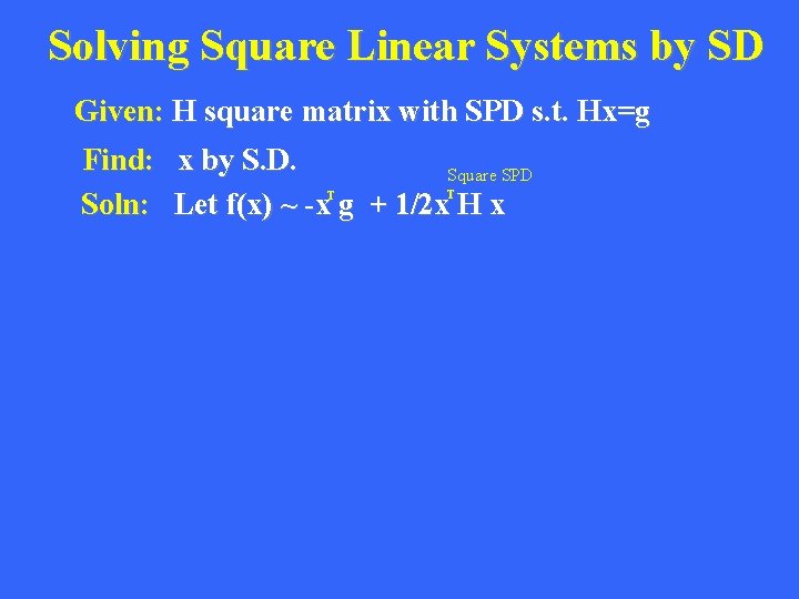
Solving Square Linear Systems by SD Given: H square matrix with SPD s. t. Hx=g Find: x by S. D. Square SPD Soln: Let f(x) ~ -x g + 1/2 x H x T T D Step 1: Set f(x)=0 Step 2: Iterative Steepest Descent (k+1) (k) x = x – a [H x - g] (k)

Outline • • • Regularized Newton Method Trust Region Method for Line Search Solving Linear System of Equations Rectangular & Regularization Traveltime Tomography Conjugate Gradient Method

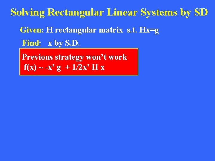
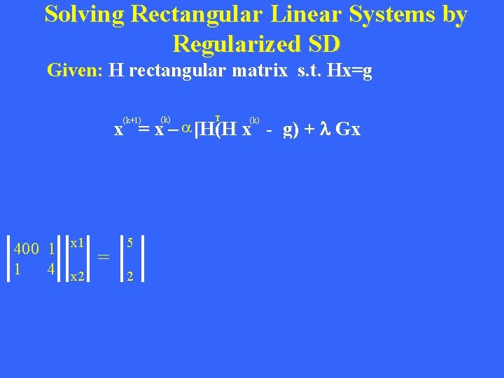
Solving Rectangular Linear Systems by SD Given: H rectangular matrix s. t. Hx=g Find: x by S. D. Soln: Letstrategy f(x) ~ 1/2 won’t (H x-g) (Hx-g) Previous work f(x) ~ -x’ g + 1/2 x’ H x Step 1: Set f(x)=0 T D Step 2: Iterative Steepest Descent Square SPD (k+1) (k) T x = x – a H(H x - g) (k) residual

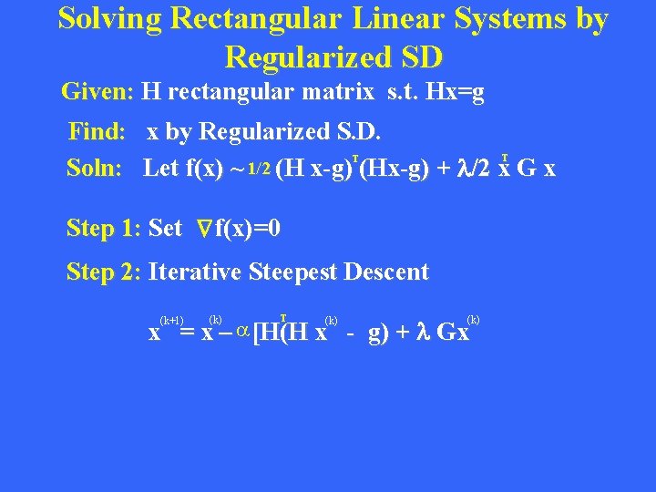
Solving Rectangular Linear Systems by Regularized SD Given: H rectangular matrix s. t. Hx=g Find: x by Regularized S. D. Soln: Let f(x) ~ 1/2 (H x-g) (Hx-g) + l/2 x G x T T D Step 1: Set f(x)=0 Step 2: Iterative Steepest Descent T x = x – a [H(H x - g) + l Gx (k+1) (k) (k) Gradient or residual Adjoint applied to residual (diff. between pred. & observed) Migration of residual

Solving Rectangular Linear Systems by Regularized SD Given: H rectangular matrix s. t. Hx=g T x = x – a [H(H x - g) + l Gx (k+1) 400 1 x 1 1 4 x 2 = 5 2 (k)

Outline • • • Regularized Newton Method Trust Region Method for Line Search Solving Linear System of Equations Rectangular & Regularization& Traveltime Tomography Scaling Conjugate Gradient Method

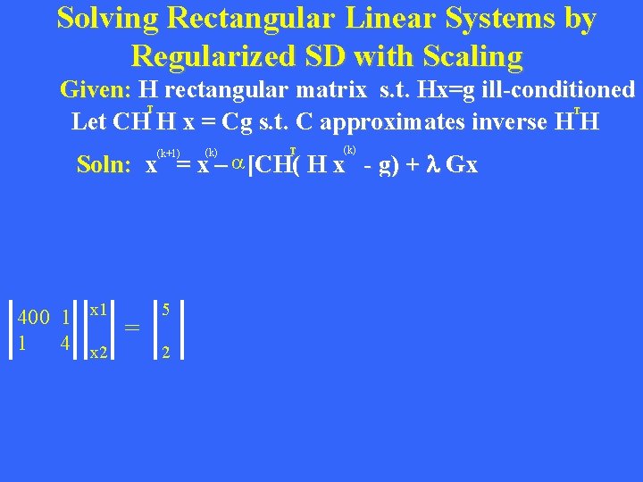
Solving Rectangular Linear Systems by Regularized SD with Scaling Given: H rectangular matrix s. t. Hx=g ill-conditioned Let CH H x = Cg s. t. C approximates inverse H H T T T (k) Soln: x = x – a [CH( H x - g) + l Gx (k+1) 400 1 x 1 1 4 x 2 = 5 2 (k)

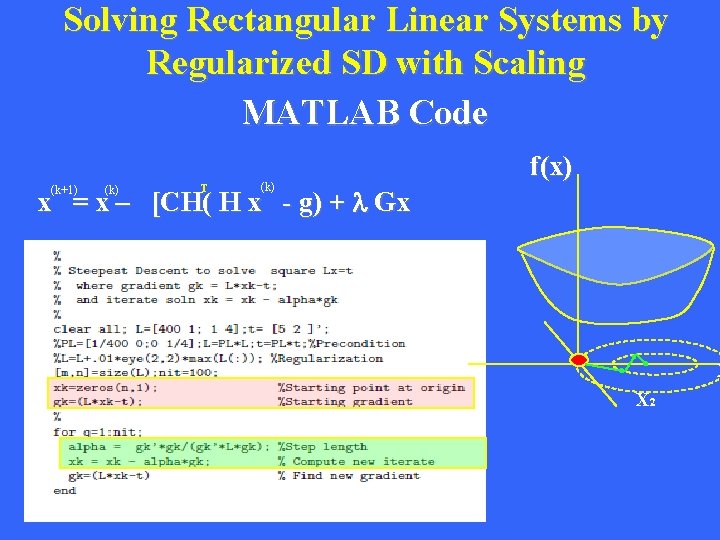
Solving Rectangular Linear Systems by Regularized SD with Scaling MATLAB Code T (k) f(x) x = x – [CH( H x - g) + l Gx (k+1) (k) X X 2

Outline • • • Regularized Newton Method Trust Region Method for Line Search Solving Linear System of Equations Traveltime Tomography Conjugate Gradient Method

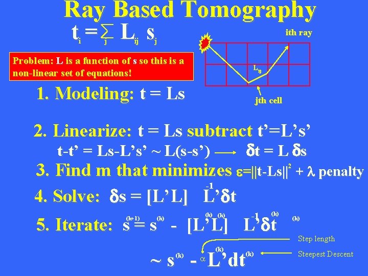
Ray Based Tomography t= L s i j ij ith ray j Problem: L is a function of s so this is a non-linear set of equations! L ij 1. Modeling: t = Ls jth cell 2. Linearize: t = Ls subtract t’=L’s’ dt = L ds t-t’ = Ls-L’s’ ~ L(s-s’) 3. Find m that minimizes e=||t-Ls|| -1 4. Solve: ds = [L’L] L’dt 2 -1 (k) (k) 5. Iterate: s = s - [L’L] L’dt (k+1) (k) ~ s - L’dt (k) a (k) + l penalty (k) Step length Steepest Descent

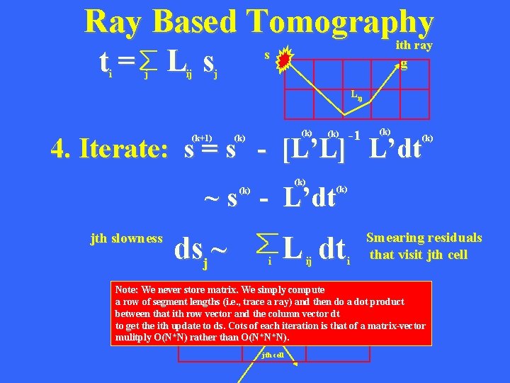
Ray Based Tomography t= L s i j ij ith ray s g j L ij (k) -1 (k) 4. Iterate: s = s - [L’L] L’dt (k+1) (k) (k) ~ s - L’dt (k) jth slowness dsj ~ i (k) L dt ij i Smearing residuals that visit jth cell Note: We never store matrix. We simply compute a row of segment lengths (i. e. , trace a ray) and then do a dot product between that ith row vector and the column vector dt to get the ith update to ds. Cots of each iteration is that of a matrix-vector mulitply O(N*N) rather than O(N*N*N). jth cell

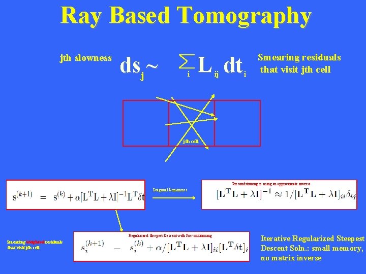
Ray Based Tomography jth slowness dsj ~ i L dt ij i Smearing residuals that visit jth cell Preconditioning is using an approximate inverse Diagonal Dominance Regularized Steepest Descent with Preconditioning Smearing weighted residuals that visit jth cell Iterative Regularized Steepest Descent Soln. : small memory, no matrix inverse

# picks Multiscale Traveltime Inversion Line 1 – Intermediate Models 1 & 2 and Final Model # unknowns (Schedule 1 -3) M=3 N>N Coarse-grain Model Intermediate Model 1 Schedule 1 Intermed. -grain Model Intermediate Model 2 Schedule 2 Finegrain Model Final Model Schedule 3 dx < l/4

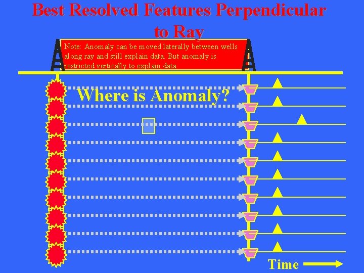
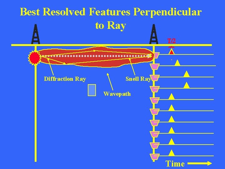
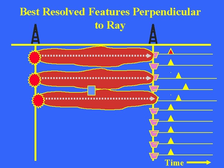
Best Resolved Features Perpendicular to Ray Note: Anomaly can be moved laterally between wells along ray and still explain data. But anomaly is restricted vertically to explain data Where is Anomaly? Time

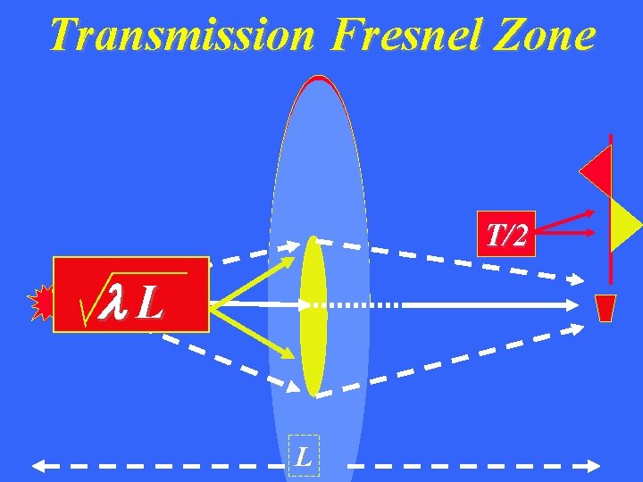
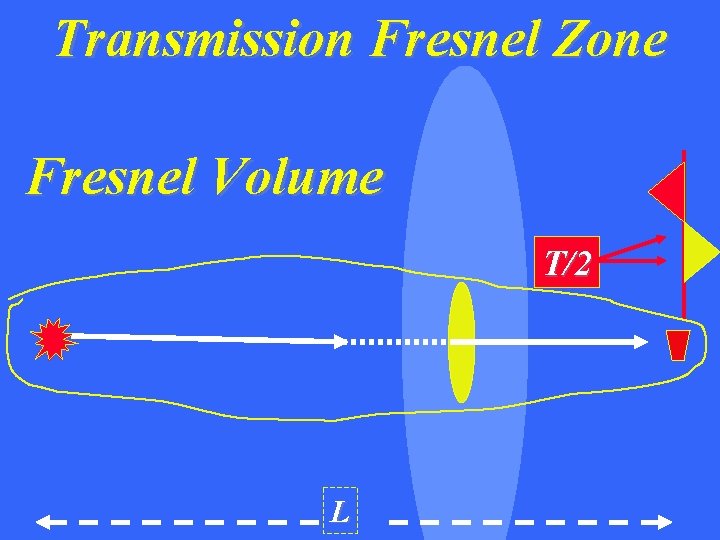
Transmission Fresnel Zone T/2 L L

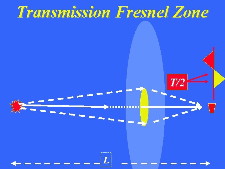
Transmission Fresnel Zone T/2 L

Transmission Fresnel Zone Fresnel Volume T/2 L

Best Resolved Features Perpendicular to Ray T/2 { Diffraction Ray Snell Ray Wavepath Time

Best Resolved Features Perpendicular to Ray Time

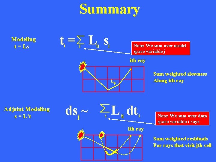
Summary Modeling t = Ls t= L s i j ij j Note: We sum over model space variable j ith ray Sum weighted slowness Along ith ray L ij Adjoint Modeling s = L’t dsj ~ i L dt ij i Note: We sum over data space variable i rays ith ray Sum weighted residuals For rays that visit jth cell

Outline • • • Regularized Newton Method Trust Region Method for Line Search Solving Linear System of Equations Traveltime Tomography Conjugate Gradient Method

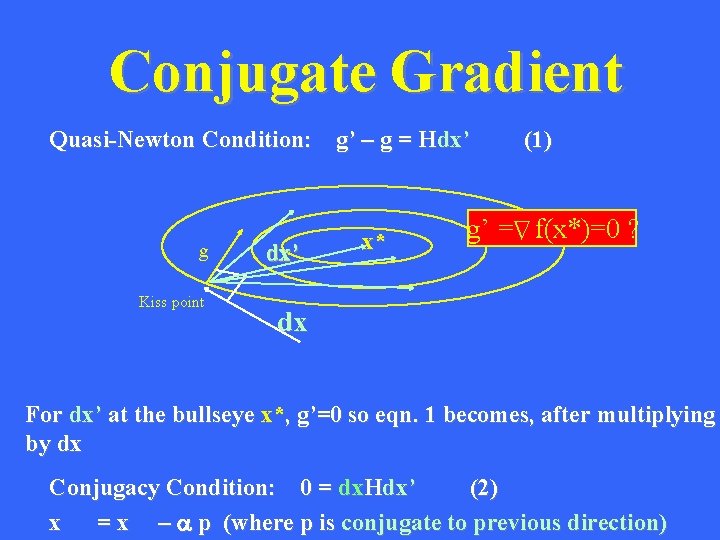
Conjugate Gradient Quasi-Newton Condition: g’ – g = Hdx’ Kiss point dx’ g’ = f(x*)=0 ? D g x* (1) dx For dx’ at the bullseye x*, g’=0 so eqn. 1 becomes, after multiplying by dx Conjugacy Condition: 0 = dx. Hdx’ (2) x = x – a p (where p is conjugate to previous direction)

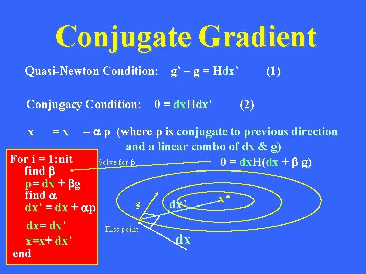
Conjugate Gradient Quasi-Newton Condition: g’ – g = Hdx’ Conjugacy Condition: 0 = dx. Hdx’ (1) (2) – a p (where p is conjugate to previous direction and a linear combo of dx & g) For i = 1: nit Solve for b 0 = dx. H(dx + b g) find b p= dx + bg find a x* g dx’ = dx + ap dx= dx’ Kiss point dx x=x+ dx’ end x =x