Statsmodels Statsmodels is a Python module that allows

Statsmodels とは • データの探索や，統計モデルの推定や，統計的な テストを行うこと可能にするモジュールである． (Statsmodels is a Python module that allows users to explore data, estimate statistical models, and perform statical test. ) URL: http: //statsmodels. sourceforge. net 理論に関しては，教科書の付録B参照 教科書 p. 187

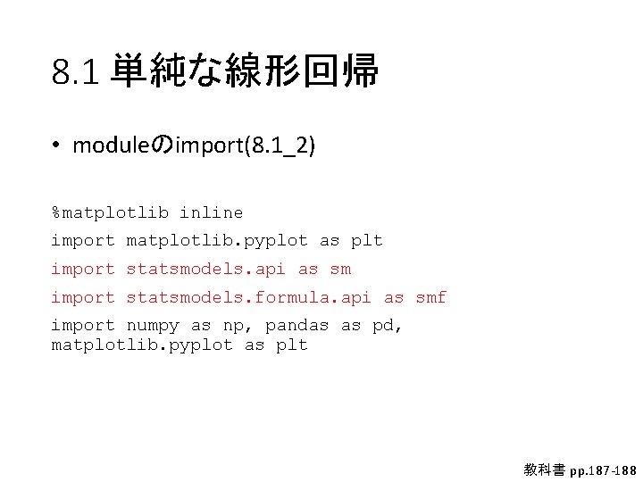
8. 1 単純な線形回帰 • moduleのimport(8. 1_2) %matplotlib inline import matplotlib. pyplot as plt import statsmodels. api as sm import statsmodels. formula. api as smf import numpy as np, pandas as pd, matplotlib. pyplot as plt 教科書 pp. 187 -188

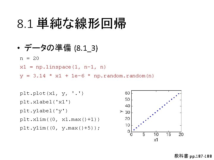
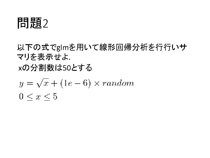
8. 1 単純な線形回帰 • データの準備 (8. 1_3) n = 20 x 1 = np. linspace(1, n-1, n) y = 3. 14 * x 1 + 1 e-6 * np. random(n) plt. plot(x 1, y, '. ') plt. xlabel('x 1') plt. ylabel('y') plt. xlim((0, x 1. max()+1)) plt. ylim((0, y. max()+5)); 教科書 pp. 187 -188

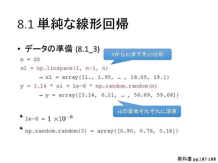
8. 1 単純な線形回帰 • データの準備 (8. 1_3) n = 20 1から19までを 20分割 x 1 = np. linspace(1, n-1, n) → x 1 = array([1. , 1. 95, … , 18. 05, 19. ]) y = 3. 14 * x 1 + 1 e-6 * np. random(n) → y = array([3. 14, 6. 11, … , 56. 69, 59. 66]) * 1 e-6 = * np. random(3) x 1の要素それぞれに演算 = array([0. 90, 0. 76, 0. 18]) 教科書 pp. 187 -188

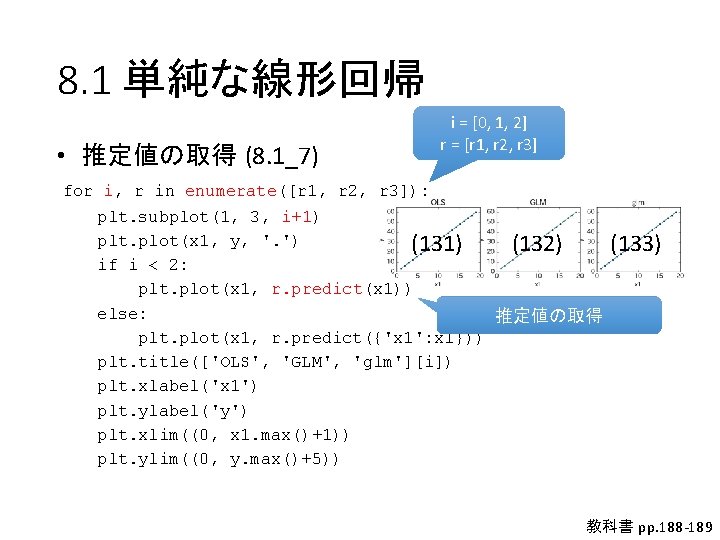
8. 1 単純な線形回帰 • 推定値の取得 (8. 1_7) for i, r in enumerate([r 1, r 2, r 3]): plt. subplot(1, 3, i+1) plt. plot(x 1, y, '. ') if i < 2: plt. plot(x 1, r. predict(x 1)) else: plt. plot(x 1, r. predict({'x 1': x 1})) plt. title(['OLS', 'GLM', 'glm'][i]) plt. xlabel('x 1') plt. ylabel('y') plt. xlim((0, x 1. max()+1)) plt. ylim((0, y. max()+5)) 教科書 pp. 188 -189

8. 1 単純な線形回帰 • 推定値の取得 (8. 1_7) i = [0, 1, 2] r = [r 1, r 2, r 3] for i, r in enumerate([r 1, r 2, r 3]): plt. subplot(1, 3, i+1) plt. plot(x 1, y, '. ') (131) (132) if i < 2: plt. plot(x 1, r. predict(x 1)) else: 推定値の取得 plt. plot(x 1, r. predict({'x 1': x 1})) plt. title(['OLS', 'GLM', 'glm'][i]) plt. xlabel('x 1') plt. ylabel('y') plt. xlim((0, x 1. max()+1)) plt. ylim((0, y. max()+5)) (133) 教科書 pp. 188 -189

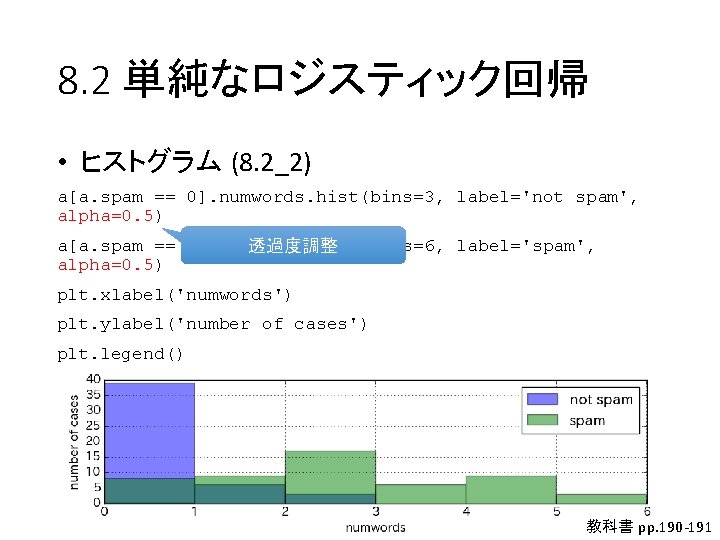
8. 2 単純なロジスティック回帰 • ヒストグラム (8. 2_2) a[a. spam == 0]. numwords. hist(bins=3, label='not spam', alpha=0. 5) a[a. spam == 1]. numwords. hist(bins=6, label='spam', alpha=0. 5) plt. xlabel('numwords') plt. ylabel('number of cases') plt. legend() 教科書 pp. 190 -191

8. 2 単純なロジスティック回帰 • ヒストグラム (8. 2_2) a[a. spam == 0]. numwords. hist(bins=3, label='not spam', alpha=0. 5) a[a. spam == 1]. numwords. hist(bins=6, label='spam', 透過度調整 alpha=0. 5) plt. xlabel('numwords') plt. ylabel('number of cases') plt. legend() 教科書 pp. 190 -191

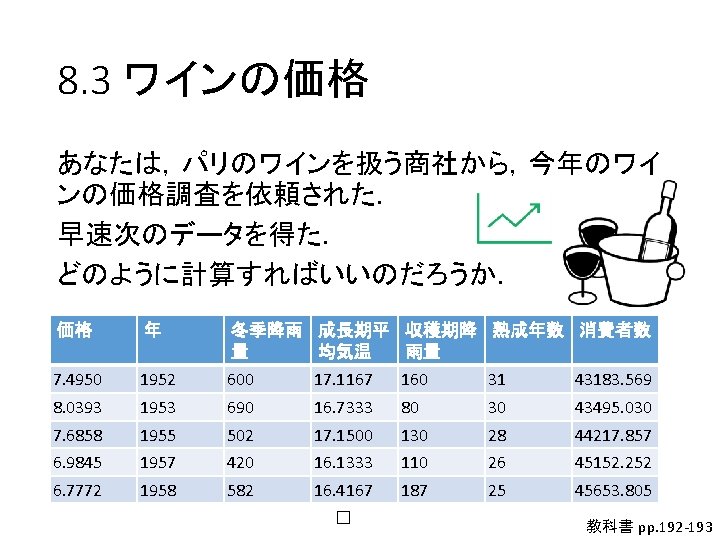
8. 3 ワインの価格 • データの準備 (8. 3. 2) import pandas as pd, numpy as np a = pd. read_csv('data/wine. csv', encoding='cp 932') a. 価格. plot(title='価格') 教科書 pp. 192 -193

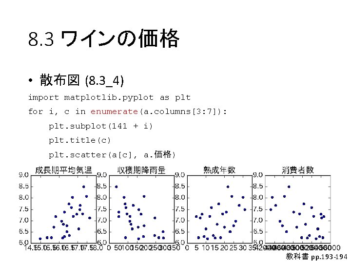
8. 3 ワインの価格 • 散布図 (8. 3_4) import matplotlib. pyplot as plt for i, c in enumerate(a. columns[3: 7]): plt. subplot(141 + i) plt. title(c) plt. scatter(a[c], a. 価格) 教科書 pp. 193 -194

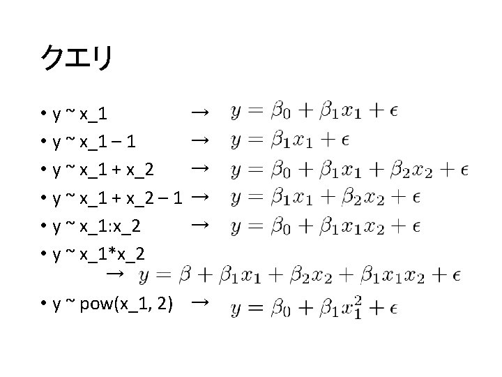
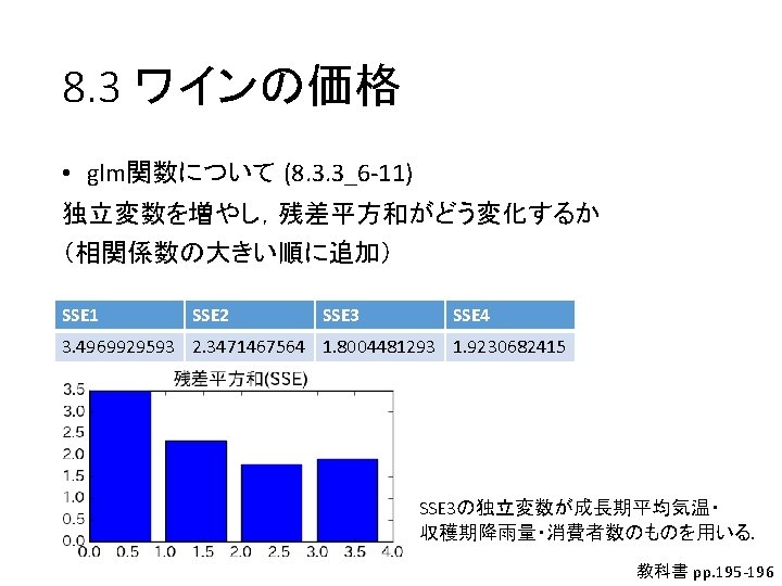
8. 3 ワインの価格 • glm関数について (8. 3. 3_6 -11) 汎用的なstatsmodels. formula. api. glm関数を用いる import statsmodels. formula. api as smf m = smf. glm('価格 ~ 成長期平均気温', a_train) r 1 = m. fit() p 1 = r 1. predict(a_test) sse 1 = np. sum((a_test. 価格 - p 1)**2) print('SSE', sse 1) 教科書 p. 195

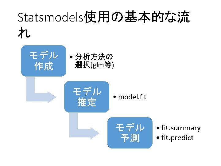
8. 3 ワインの価格 • glm関数について (8. 3. 3_6 -11) 汎用的なstatsmodels. formula. api. glm関数を用いる モデル作成 → 推定 → 予測 import statsmodels. formula. api as smf m = smf. glm('価格 ~ 成長期平均気温', a_train) r 1 = m. fit() p 1 = r 1. predict(a_test) sse 1 = np. sum((a_test. 価格 - p 1)**2) print('SSE', sse 1) 残差平方和の計算 教科書 p. 195

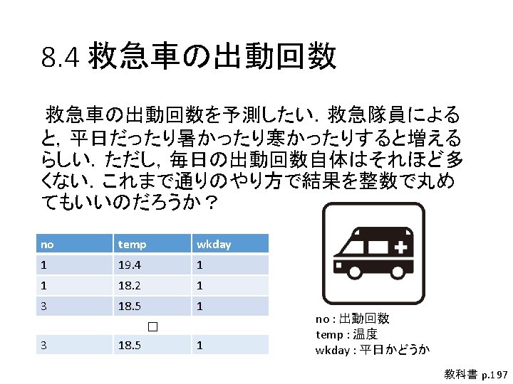
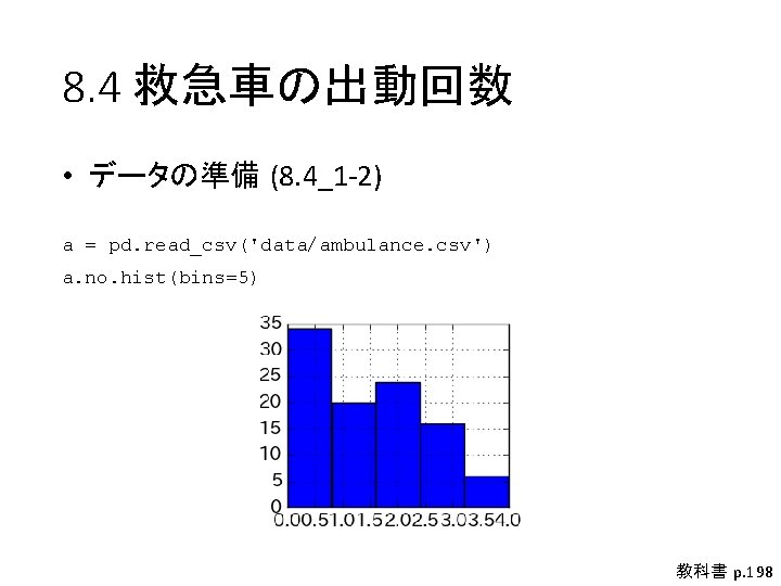
8. 4 救急車の出動回数 • データの準備 (8. 4_1 -2) a = pd. read_csv('data/ambulance. csv') a. no. hist(bins=5) 教科書 p. 198

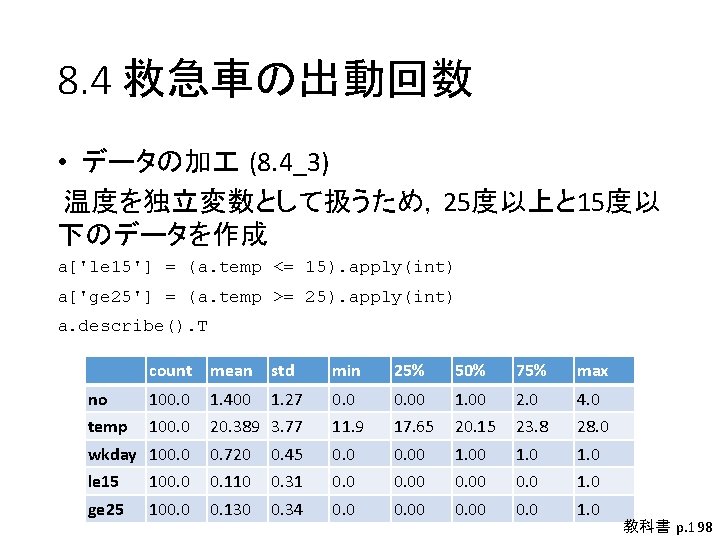
8. 4 救急車の出動回数 • データの加 (8. 4_3) 温度を独立変数として扱うため，25度以上と 15度以 下のデータを作成 a['le 15'] = (a. temp <= 15). apply(int) a['ge 25'] = (a. temp >= 25). apply(int) a. describe(). T count mean std min 25% 50% 75% max no 100. 0 1. 400 1. 27 0. 00 1. 00 2. 0 4. 0 temp 100. 0 20. 389 3. 77 11. 9 17. 65 20. 15 23. 8 28. 0 wkday 100. 0 0. 720 0. 45 0. 00 1. 0 le 15 100. 0 0. 110 0. 31 0. 00 0. 0 1. 0 ge 25 100. 0 0. 130 0. 34 0. 00 0. 0 1. 0 教科書 p. 198

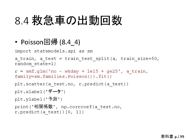
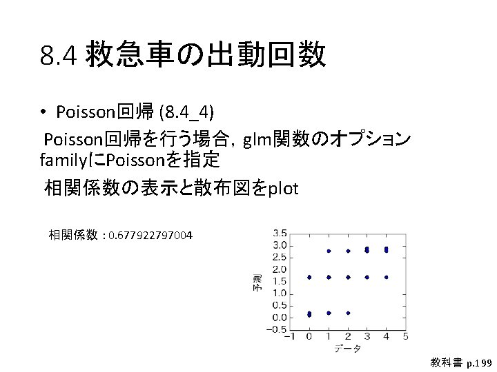
8. 4 救急車の出動回数 • Poisson回帰 (8. 4_4) import statsmodels. api as sm a_train, a_test = train_test_split(a, train_size=50, random_state=1) r = smf. glm('no ~ wkday + le 15 + ge 25', a_train, family=sm. families. Poisson()). fit() plt. scatter(a_test. no, r. predict(a_test)) plt. xlabel('データ') plt. ylabel('予測') print('相関係数', np. corrcoef(a_test. no, r. predict(a_test))[0, 1]) 教科書 p. 199

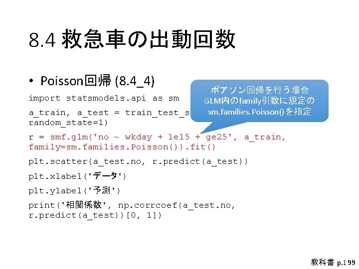
8. 4 救急車の出動回数 • Poisson回帰 (8. 4_4) ポアソン回帰を行う場合 import statsmodels. api as sm GLM内のfamily引数に規定の sm. families. Poisson()を指定 a_train, a_test = train_test_split(a, train_size=50, random_state=1) r = smf. glm('no ~ wkday + le 15 + ge 25', a_train, family=sm. families. Poisson()). fit() plt. scatter(a_test. no, r. predict(a_test)) plt. xlabel('データ') plt. ylabel('予測') print('相関係数', np. corrcoef(a_test. no, r. predict(a_test))[0, 1]) 教科書 p. 199

8. 5 医療の質 • データの準備 (8. 5_1) データを読み込みColumnデータを表示 a = pd. read_csv('data/quality. csv', index_col=0) for c in a. columns[: -1]: print(c) 教科書 p. 200

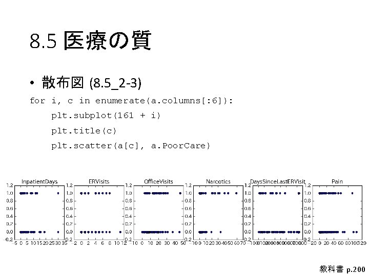
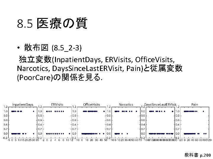
8. 5 医療の質 • 散布図 (8. 5_2 -3) for i, c in enumerate(a. columns[: 6]): plt. subplot(161 + i) plt. title(c) plt. scatter(a[c], a. Poor. Care) 教科書 p. 200

8. 5 医療の質 • 散布図 (8. 5_2 -3) 独立変数(Inpatient. Days, ERVisits, Office. Visits, Narcotics, Days. Since. Last. ERVisit, Pain)と従属変数 (Poor. Care)の関係を見る． 教科書 p. 200

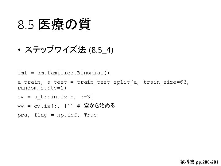
8. 5 医療の質 • ステップワイズ法 (8. 5_4) fml = sm. families. Binomial() a_train, a_test = train_test_split(a, train_size=66, random_state=1) cv = a_train. ix[: , : -3] vv = cv. ix[: , []] # 空から始める pra, flag = np. inf, True 教科書 pp. 200 -201

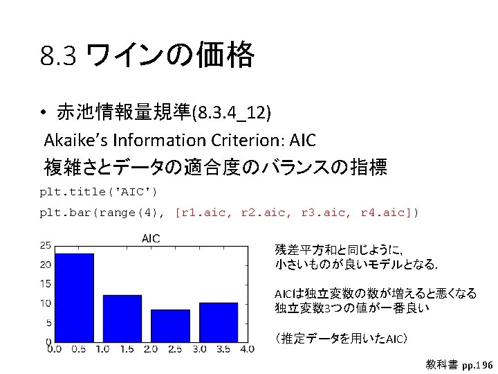
ステップワイズ法 (8. 5_4) # 更新がない場合終了 while flag and len(vv. columns) < len(cv. columns): flag, best = False, None # 追加のループ for c in cv: if c not in vv: # 独立変数が入っていない場合 # AICの確認 vv[c] = cv[c] r = sm. GLM(a_train. Poor. Care, vv, family=fml). fit() vv. drop(c, axis=1, inplace=True) if r. aic < pra: # 改善した場合 flag, best, pra = True, c, r. aic if best: # 一度でもAICが改善した場合 vv[best] = cv[best] 教科書 pp. 200 -201

ステップワイズ法 (8. 5_4) best = True # 削除のループ, 更新が無い場合終了 while best and len(vv. columns) > 1: best = None for c in vv: # AICの確認 vv. drop(c, axis=1, inplace=True) r = sm. GLM(a_train. Poor. Care, vv, family=fml). fit() vv[c] = cv[c] if r. aic < pra: # 改善した場合 flag, best, pref = True, c, r. aic if best: # 一度でも改善した場合 vv. drop(best, axis=1, inplace=True) 教科書 pp. 200 -201

8. 5 医療の質 • 結果の確認 (8. 5_5 -6) r = sm. GLM(a_train. Poor. Care, vv, family=fml). fit() p = r. predict(a_test[vv. columns]) print('相関係数', np. corrcoef(a_test. Poor. Care, p)[0, 1]) print('SSE', np. sum((a_test. Poor. Care - p)**2)) plt. scatter(a_test. Poor. Care, p) plt. xlabel('データ') plt. ylabel('予測') 相関係数 : 0. 302083672512 SSE : 14. 4166494065637 教科書 pp. 201 -202