Stats 330 Lecture 26 Department of Statistics 2012

Stats 330: Lecture 26 © Department of Statistics 2012 STATS 330 Lecture 26: Slide 1

Plan of the day In today’s lecture we begin our discussion of Poisson regression Topics – The Poisson regression model – Three examples © Department of Statistics 2012 STATS 330 Lecture 26: Slide 2

Poisson regression So far we have looked at 2 kinds of regression • “Normal regression” – Continuous response, normally distributed with constant variance – Mean a linear function of the covariates • “Logistic regression” – Response (number of successes in n trials) has a binomial distribution Bin(n, p) – Mean is np where log-odds of p is a linear function of the covariates © Department of Statistics 2012 STATS 330 Lecture 26: Slide 3

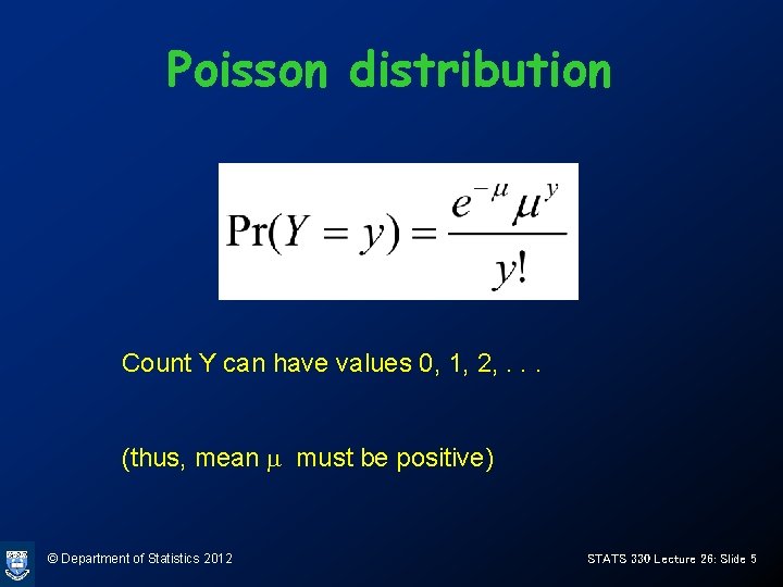
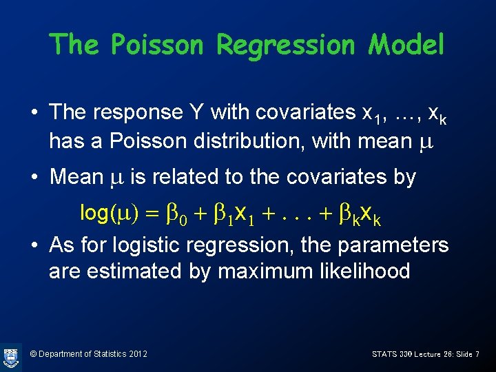
Poisson regression (cont) • Now we consider “Poisson regression” – Response is a count, assumed to have a Poisson distribution with (positive) mean m – Assume that log m is a linear function of the covariates – Alternatively, m = exp( linear function of covariates) • Poisson is a standard distribution when response is a count. © Department of Statistics 2012 STATS 330 Lecture 26: Slide 4

Poisson distribution Count Y can have values 0, 1, 2, . . . (thus, mean m must be positive) © Department of Statistics 2012 STATS 330 Lecture 26: Slide 5

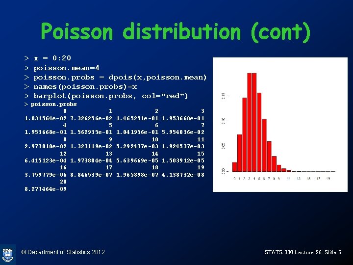
Poisson distribution (cont) > > > x = 0: 20 poisson. mean=4 poisson. probs = dpois(x, poisson. mean) names(poisson. probs)=x barplot(poisson. probs, col="red") > poisson. probs 0 1 1. 831564 e-02 7. 326256 e-02 4 5 1. 953668 e-01 1. 562935 e-01 8 9 2. 977018 e-02 1. 323119 e-02 12 13 6. 415123 e-04 1. 973884 e-04 16 17 3. 759779 e-06 8. 846539 e-07 20 8. 277464 e-09 © Department of Statistics 2012 2 1. 465251 e-01 6 1. 041956 e-01 10 5. 292477 e-03 14 5. 639669 e-05 18 1. 965898 e-07 3 1. 953668 e-01 7 5. 954036 e-02 11 1. 924537 e-03 15 1. 503912 e-05 19 4. 138732 e-08 STATS 330 Lecture 26: Slide 6

The Poisson Regression Model • The response Y with covariates x 1, …, xk has a Poisson distribution, with mean m • Mean m is related to the covariates by log(m) = b 0 + b 1 x 1 +. . . + bkxk • As for logistic regression, the parameters are estimated by maximum likelihood © Department of Statistics 2012 STATS 330 Lecture 26: Slide 7

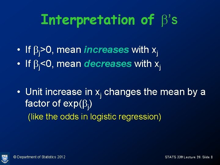
Interpretation of b’s • If bj>0, mean increases with xj • If bj<0, mean decreases with xj • Unit increase in xj changes the mean by a factor of exp(bj) (like the odds in logistic regression) © Department of Statistics 2012 STATS 330 Lecture 26: Slide 8

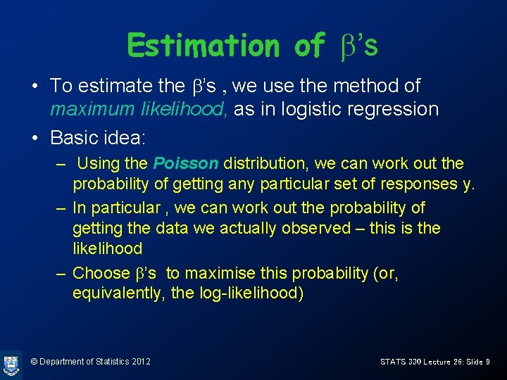
Estimation of b’s • To estimate the b’s , we use the method of maximum likelihood, as in logistic regression • Basic idea: – Using the Poisson distribution, we can work out the probability of getting any particular set of responses y. – In particular , we can work out the probability of getting the data we actually observed – this is the likelihood – Choose b’s to maximise this probability (or, equivalently, the log-likelihood) © Department of Statistics 2012 STATS 330 Lecture 26: Slide 9

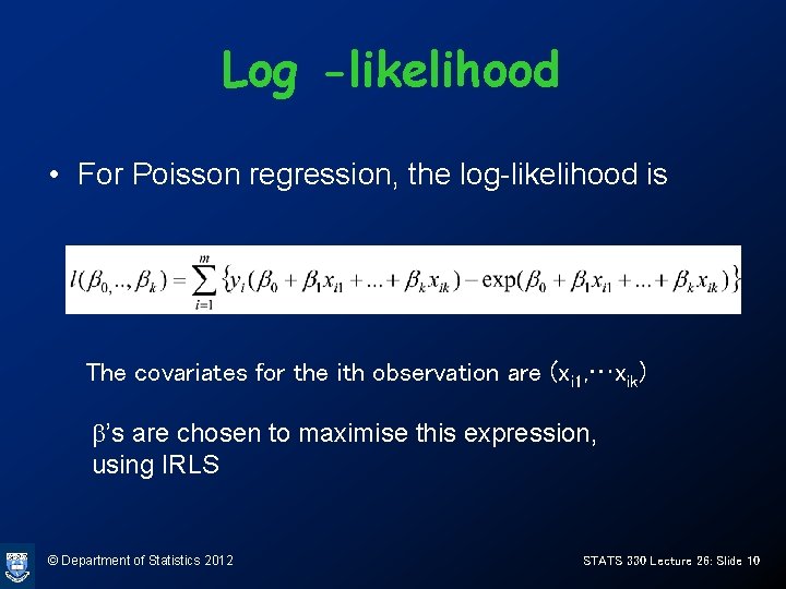
Log -likelihood • For Poisson regression, the log-likelihood is The covariates for the ith observation are (xi 1, …xik) b’s are chosen to maximise this expression, using IRLS © Department of Statistics 2012 STATS 330 Lecture 26: Slide 10

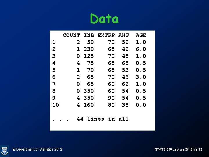
Example: Mining accident data • This example features the number of accidents per mine in a 3 month period in 44 coal mines in West Virginia. The variables are – COUNT: the number of accidents (response) – INB: inner burden thickness – EXTRP: percentage of coal extracted from mine – AHS: the average height of the coal seam in the mine – AGE: the age of the mine © Department of Statistics 2012 STATS 330 Lecture 26: Slide 11

Data COUNT 1 2 2 1 3 0 4 4 5 1 6 2 7 0 8 0 9 4 10 4. . . © Department of Statistics 2012 INB EXTRP AHS 50 70 52 230 65 42 125 70 45 75 65 68 70 65 53 65 70 46 65 60 62 350 60 54 350 90 54 160 80 38 AGE 1. 0 6. 0 1. 0 0. 5 3. 0 1. 0 0. 5 0. 0 44 lines in all STATS 330 Lecture 26: Slide 12

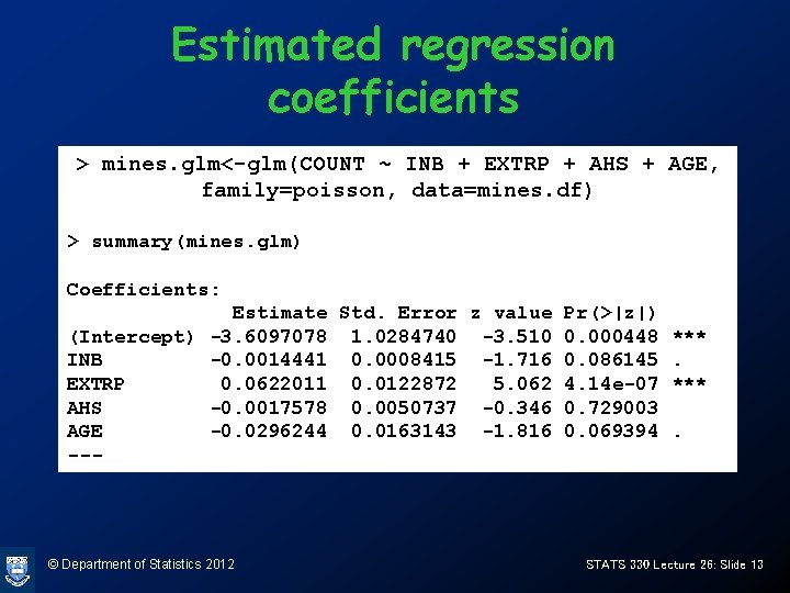
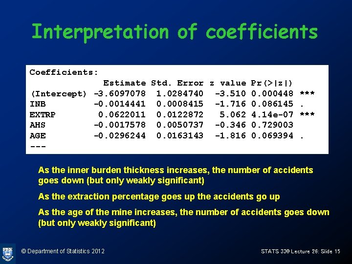
Estimated regression coefficients > mines. glm<-glm(COUNT ~ INB + EXTRP + AHS + AGE, family=poisson, data=mines. df) > summary(mines. glm) Coefficients: Estimate Std. Error z value Pr(>|z|) (Intercept) -3. 6097078 1. 0284740 -3. 510 0. 000448 *** INB -0. 0014441 0. 0008415 -1. 716 0. 086145. EXTRP 0. 0622011 0. 0122872 5. 062 4. 14 e-07 *** AHS -0. 0017578 0. 0050737 -0. 346 0. 729003 AGE -0. 0296244 0. 0163143 -1. 816 0. 069394. --- © Department of Statistics 2012 STATS 330 Lecture 26: Slide 13

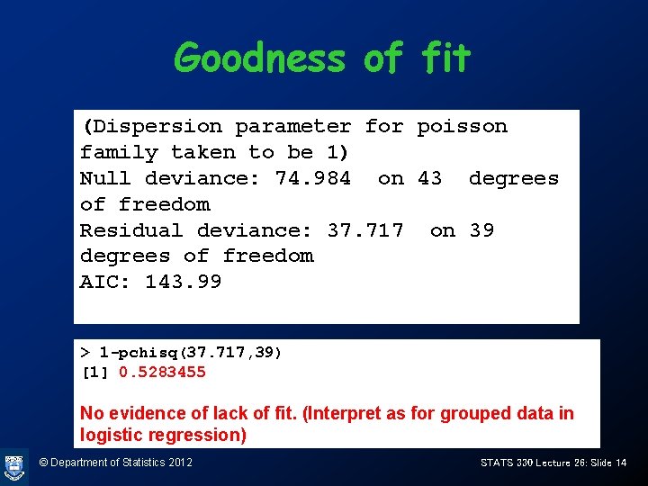
Goodness of fit (Dispersion parameter for poisson family taken to be 1) Null deviance: 74. 984 on 43 degrees of freedom Residual deviance: 37. 717 on 39 degrees of freedom AIC: 143. 99 > 1 -pchisq(37. 717, 39) [1] 0. 5283455 No evidence of lack of fit. (Interpret as for grouped data in logistic regression) © Department of Statistics 2012 STATS 330 Lecture 26: Slide 14

Interpretation of coefficients Coefficients: Estimate Std. Error z value Pr(>|z|) (Intercept) -3. 6097078 1. 0284740 -3. 510 0. 000448 *** INB -0. 0014441 0. 0008415 -1. 716 0. 086145. EXTRP 0. 0622011 0. 0122872 5. 062 4. 14 e-07 *** AHS -0. 0017578 0. 0050737 -0. 346 0. 729003 AGE -0. 0296244 0. 0163143 -1. 816 0. 069394. --As the inner burden thickness increases, the number of accidents goes down (but only weakly significant) As the extraction percentage goes up the accidents go up As the age of the mine increases, the number of accidents goes down (but only weakly significant) © Department of Statistics 2012 STATS 330 Lecture 26: Slide 15

Example: Onions • These data come from an onion-growing experiment at the Hort Research station at Pukekohe. • The experiment was conducted to compare the effect of different methods of “curing” on the number of skins on individual onions at different stages of maturity. © Department of Statistics 2012 STATS 330 Lecture 26: Slide 16

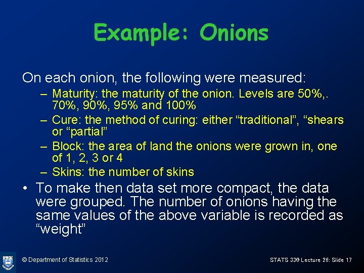
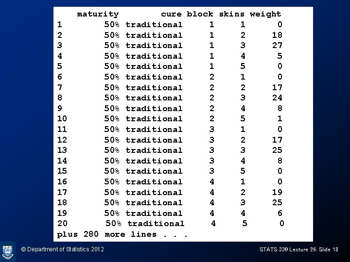
Example: Onions On each onion, the following were measured: – Maturity: the maturity of the onion. Levels are 50%, . 70%, 95% and 100% – Cure: the method of curing: either “traditional”, “shears or “partial” – Block: the area of land the onions were grown in, one of 1, 2, 3 or 4 – Skins: the number of skins • To make then data set more compact, the data were grouped. The number of onions having the same values of the above variable is recorded as “weight” © Department of Statistics 2012 STATS 330 Lecture 26: Slide 17

maturity cure block skins weight 1 50% traditional 1 1 0 2 50% traditional 1 2 18 3 50% traditional 1 3 27 4 50% traditional 1 4 5 5 50% traditional 1 5 0 6 50% traditional 2 1 0 7 50% traditional 2 2 17 8 50% traditional 2 3 24 9 50% traditional 2 4 8 10 50% traditional 2 5 1 11 50% traditional 3 1 0 12 50% traditional 3 2 17 13 50% traditional 3 3 25 14 50% traditional 3 4 8 15 50% traditional 3 5 0 16 50% traditional 4 1 0 17 50% traditional 4 2 19 18 50% traditional 4 3 25 19 50% traditional 4 4 6 20 50% traditional 4 5 0 plus 280 more lines. . . © Department of Statistics 2012 STATS 330 Lecture 26: Slide 18

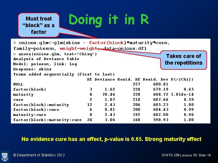
Must treat “block” as a factor Doing it in R > onions. glm<-glm(skins ~ factor(block)*maturity*cure, family=poisson, weight=weight, data=onions. df) > anova(onions. glm, test="Chisq") Takes care of Analysis of Deviance Table the repetitions Model: poisson, link: log Response: skins Terms added sequentially (first to last) Df Deviance Resid. Df Resid. Dev P(>|Chi|) NULL 227 680. 81 factor(block) 3 1. 62 224 679. 19 0. 65 maturity 4 70. 46 220 608. 72 1. 814 e-14 cure 2 1. 07 218 607. 66 0. 59 factor(block): maturity 12 2. 43 206 605. 23 1. 00 factor(block): cure 6 0. 81 200 604. 43 0. 99 maturity: cure 8 2. 43 192 602. 00 0. 96 factor(block): maturity: cure 24 3. 06 168 598. 93 1. 00 No evidence cure has an effect, p-value is 0. 65. Strong maturity effect © Department of Statistics 2012 STATS 330 Lecture 26: Slide 19

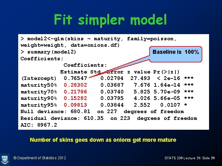
Fit simpler model > model 2<-glm(skins ~ maturity, family=poisson, weight=weight, data=onions. df) > summary(model 2) Baseline is 100% Coefficients: Estimate Std. Error z value Pr(>|z|) (Intercept) 0. 76547 0. 02784 27. 493 < 2 e-16 *** maturity 50% 0. 28302 0. 03687 7. 676 1. 64 e-14 *** maturity 70% 0. 21786 0. 03740 5. 825 5. 70 e-09 *** maturity 90% 0. 15282 0. 03795 4. 026 5. 66 e-05 *** maturity 95% 0. 09813 0. 03844 2. 552 0. 0107 * Null deviance: 680. 81 on 227 degrees of freedom Residual deviance: 610. 35 on 223 degrees of freedom AIC: 8967. 2 Number of skins goes down as onions get more mature © Department of Statistics 2012 STATS 330 Lecture 26: Slide 20

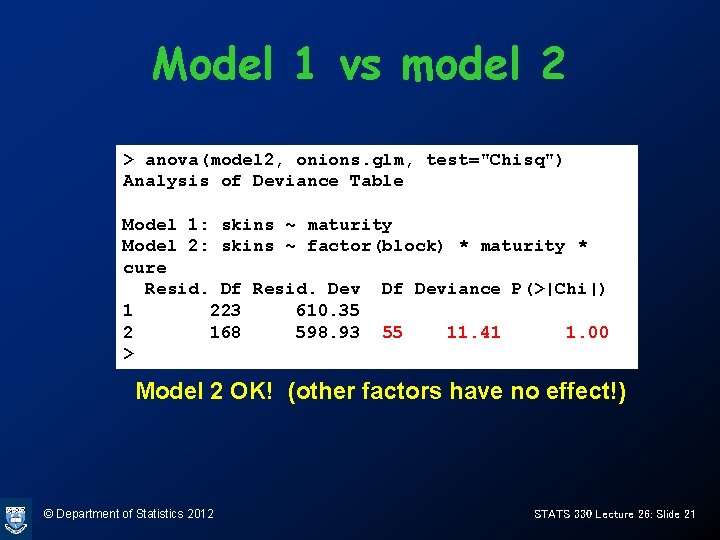
Model 1 vs model 2 > anova(model 2, onions. glm, test="Chisq") Analysis of Deviance Table Model 1: skins ~ maturity Model 2: skins ~ factor(block) * maturity * cure Resid. Df Resid. Dev Df Deviance P(>|Chi|) 1 223 610. 35 2 168 598. 93 55 11. 41 1. 00 > Model 2 OK! (other factors have no effect!) © Department of Statistics 2012 STATS 330 Lecture 26: Slide 21

Offsets • Often Poisson data are concerned with rates, as in death rates or accident rates in a population. • In this case, we look at the number of deaths from a particular cause over a period of time. The number of deaths will be related to the population size, and the time, which we have to take into account. • We could treat the data as binomial, but a more common approach is to use offsets. © Department of Statistics 2012 STATS 330 Lecture 26: Slide 22

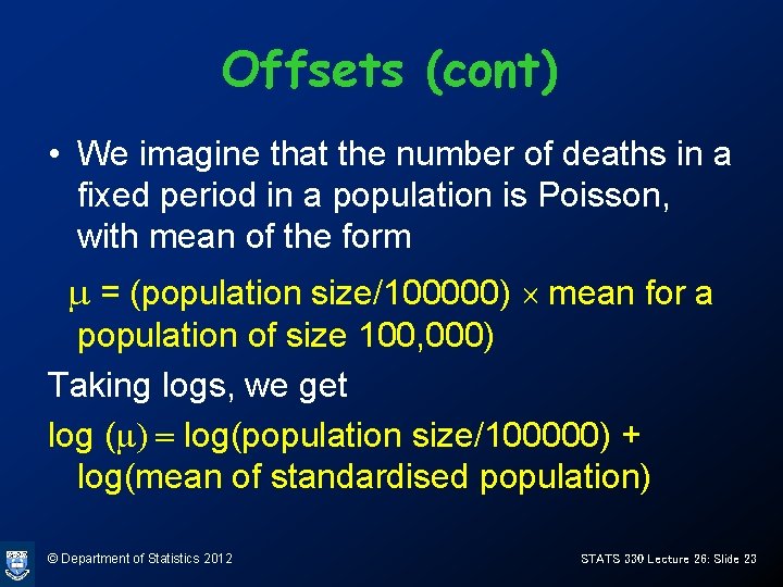
Offsets (cont) • We imagine that the number of deaths in a fixed period in a population is Poisson, with mean of the form m = (population size/100000) ´ mean for a population of size 100, 000) Taking logs, we get log (m) = log(population size/100000) + log(mean of standardised population) © Department of Statistics 2012 STATS 330 Lecture 26: Slide 23

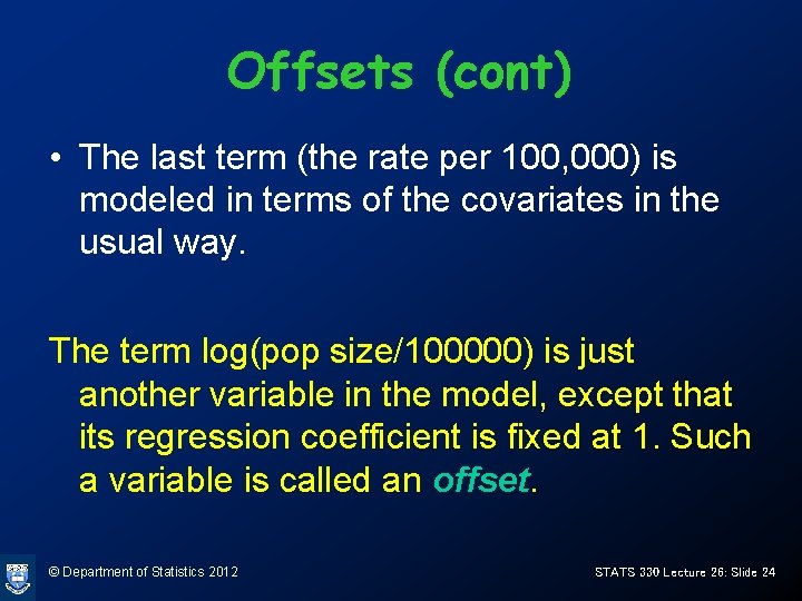
Offsets (cont) • The last term (the rate per 100, 000) is modeled in terms of the covariates in the usual way. The term log(pop size/100000) is just another variable in the model, except that its regression coefficient is fixed at 1. Such a variable is called an offset. © Department of Statistics 2012 STATS 330 Lecture 26: Slide 24

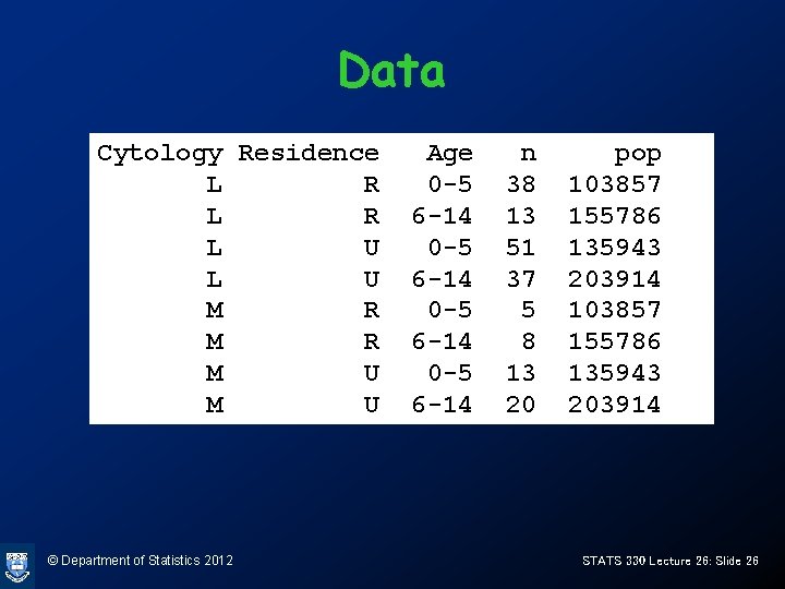
Example • Deaths from childhood cancers 1951 – 1960 in Northumberland Durham, classified by – Cytology (Lymphoblastic / Myeloblastic) – Residence (Rural/Urban) – Age (0 -5, 6 -14) © Department of Statistics 2012 STATS 330 Lecture 26: Slide 25

Data Cytology Residence L R L U M R M U © Department of Statistics 2012 Age 0 -5 6 -14 n 38 13 51 37 5 8 13 20 pop 103857 155786 135943 203914 STATS 330 Lecture 26: Slide 26

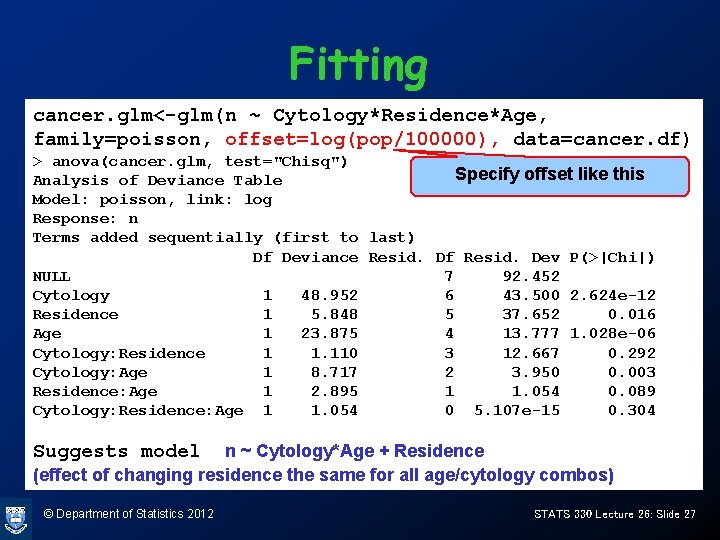
Fitting cancer. glm<-glm(n ~ Cytology*Residence*Age, family=poisson, offset=log(pop/100000), data=cancer. df) > anova(cancer. glm, test="Chisq") Specify offset like this Analysis of Deviance Table Model: poisson, link: log Response: n Terms added sequentially (first to last) Df Deviance Resid. Df Resid. Dev P(>|Chi|) NULL 7 92. 452 Cytology 1 48. 952 6 43. 500 2. 624 e-12 Residence 1 5. 848 5 37. 652 0. 016 Age 1 23. 875 4 13. 777 1. 028 e-06 Cytology: Residence 1 1. 110 3 12. 667 0. 292 Cytology: Age 1 8. 717 2 3. 950 0. 003 Residence: Age 1 2. 895 1 1. 054 0. 089 Cytology: Residence: Age 1 1. 054 0 5. 107 e-15 0. 304 Suggests model n ~ Cytology*Age + Residence (effect of changing residence the same for all age/cytology combos) © Department of Statistics 2012 STATS 330 Lecture 26: Slide 27

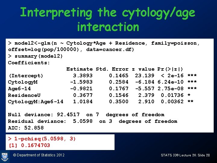
Interpreting the cytology/age interaction > model 2<-glm(n ~ Cytology*Age + Residence, family=poisson, offset=log(pop/100000), data=cancer. df) > summary(model 2) Coefficients: Estimate Std. Error z value Pr(>|z|) (Intercept) 3. 3893 0. 1465 23. 139 < 2 e-16 *** Cytology. M -1. 5983 0. 2584 -6. 184 6. 24 e-10 *** Age 6 -14 -0. 9821 0. 1767 -5. 557 2. 75 e-08 *** Residence. U 0. 3677 0. 1546 2. 379 0. 01736 * Cytology. M: Age 6 -14 1. 0184 0. 3500 2. 910 0. 00362 ** Null deviance: 92. 4517 on 7 degrees of freedom Residual deviance: 5. 0598 on 3 degrees of freedom AIC: 52. 858 > 1 -pchisq(5. 0598, 3) [1] 0. 1674703 © Department of Statistics 2012 STATS 330 Lecture 26: Slide 28

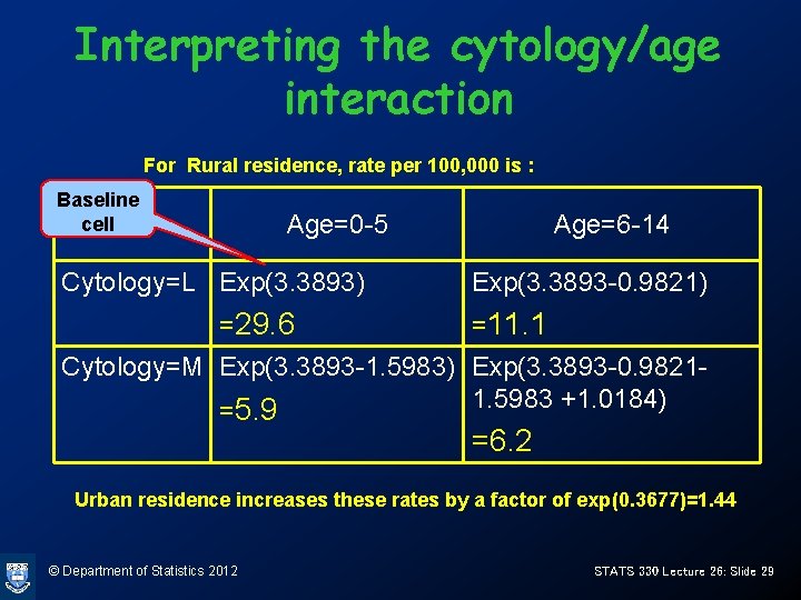
Interpreting the cytology/age interaction For Rural residence, rate per 100, 000 is : Baseline cell Age=0 -5 Cytology=L Exp(3. 3893) =29. 6 Age=6 -14 Exp(3. 3893 -0. 9821) =11. 1 Cytology=M Exp(3. 3893 -1. 5983) Exp(3. 3893 -0. 98211. 5983 +1. 0184) =5. 9 =6. 2 Urban residence increases these rates by a factor of exp(0. 3677)=1. 44 © Department of Statistics 2012 STATS 330 Lecture 26: Slide 29