Stats 330 Lecture 22 Department of Statistics 2012



- Slides: 33

Stats 330: Lecture 22 © Department of Statistics 2012 STATS 330 Lecture 22: Slide 1

Plan of the day In today’s lecture we continue our discussion of the logistic regression model Topics covered – Multiple logistic regression – Grouped data in multiple linear regression – Deviances – Models and submodels Reference: Coursebook, sections 5. 2. 3, 5. 2. 4 © Department of Statistics 2012 STATS 330 Lecture 22: Slide 2

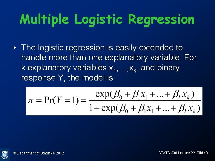
Multiple Logistic Regression • The logistic regression is easily extended to handle more than one explanatory variable. For k explanatory variables x 1, …, xk, and binary response Y, the model is © Department of Statistics 2012 STATS 330 Lecture 22: Slide 3

Odds & log-odds form © Department of Statistics 2012 STATS 330 Lecture 22: Slide 4

Interpretation of coefficients • As before, a unit increase in xj multiplies the odds by exp(bj) • A unit increase in xj adds bj to the log-odds © Department of Statistics 2012 STATS 330 Lecture 22: Slide 5

Grouped and ungrouped data in multiple LR • To group two individuals in multiple LR, the individuals must have the same values for all the covariates • Each distinct set of covariates is called a covariate pattern • If there are m distinct covariate patterns, we record for each pattern the number of individuals having that pattern (n) and the number of “successes” (r). © Department of Statistics 2012 STATS 330 Lecture 22: Slide 6

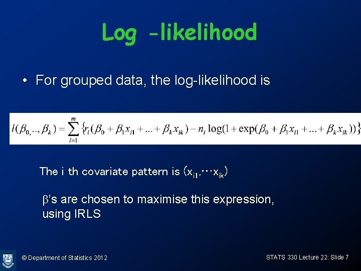
Log -likelihood • For grouped data, the log-likelihood is The i th covariate pattern is (xi 1, …xik) b’s are chosen to maximise this expression, using IRLS © Department of Statistics 2012 STATS 330 Lecture 22: Slide 7

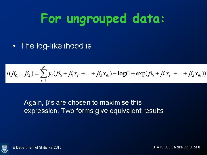
For ungrouped data: • The log-likelihood is Again, b’s are chosen to maximise this expression. Two forms give equivalent results © Department of Statistics 2012 STATS 330 Lecture 22: Slide 8

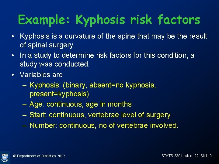
Example: Kyphosis risk factors • Kyphosis is a curvature of the spine that may be the result of spinal surgery. • In a study to determine risk factors for this condition, a study was conducted. • Variables are – Kyphosis: (binary, absent=no kyphosis, present=kyphosis) – Age: continuous, age in months – Start: continuous, vertebrae level of surgery – Number: continuous, no of vertebrae involved. © Department of Statistics 2012 STATS 330 Lecture 22: Slide 9

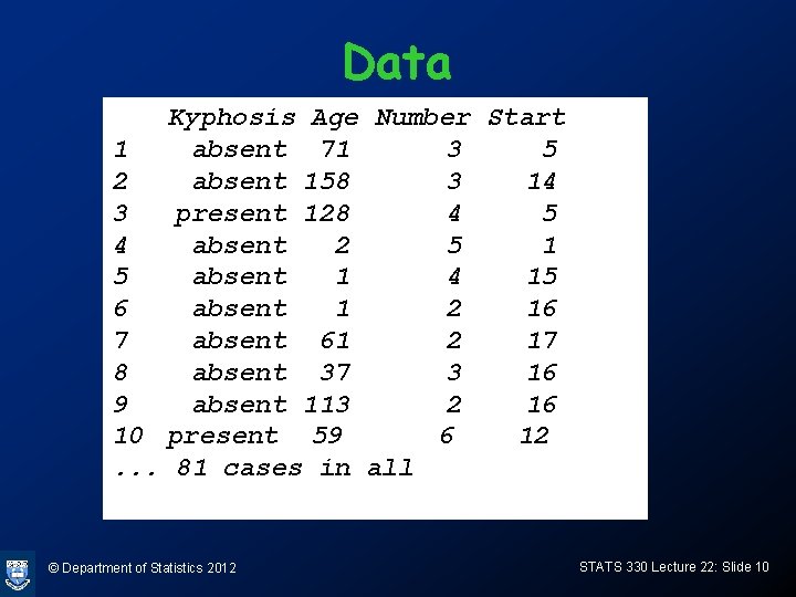
Data Kyphosis Age Number Start 1 absent 71 3 5 2 absent 158 3 14 3 present 128 4 5 4 absent 2 5 1 5 absent 1 4 15 6 absent 1 2 16 7 absent 61 2 17 8 absent 37 3 16 9 absent 113 2 16 10 present 59 6 12. . . 81 cases in all © Department of Statistics 2012 STATS 330 Lecture 22: Slide 10

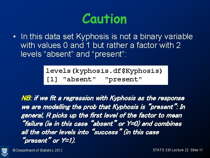
Caution • In this data set Kyphosis is not a binary variable with values 0 and 1 but rather a factor with 2 levels “absent” and “present”: levels(kyphosis. df$Kyphosis) [1] "absent" "present" NB: if we fit a regression with Kyphosis as the response we are modelling the prob that Kyphosis is “present”: In general, R picks up the first level of the factor to mean “failure (ie in this case “absent” or Y=0) and combines all the other levels into “success” (in this case “present” or Y=1). © Department of Statistics 2012 STATS 330 Lecture 22: Slide 11

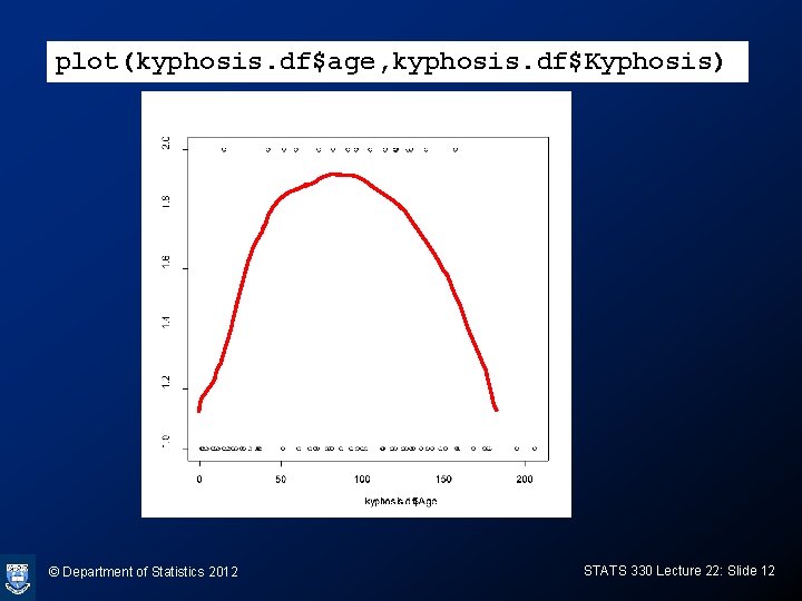
plot(kyphosis. df$age, kyphosis. df$Kyphosis) © Department of Statistics 2012 STATS 330 Lecture 22: Slide 12

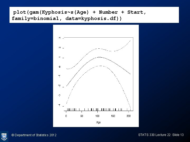
plot(gam(Kyphosis~s(Age) + Number + Start, family=binomial, data=kyphosis. df)) © Department of Statistics 2012 STATS 330 Lecture 22: Slide 13

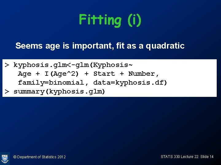
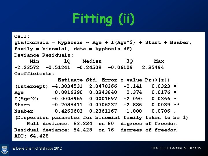
Fitting (i) Seems age is important, fit as a quadratic > kyphosis. glm<-glm(Kyphosis~ Age + I(Age^2) + Start + Number, family=binomial, data=kyphosis. df) > summary(kyphosis. glm) © Department of Statistics 2012 STATS 330 Lecture 22: Slide 14

Fitting (ii) Call: glm(formula = Kyphosis ~ Age + I(Age^2) + Start + Number, family = binomial, data = kyphosis. df) Deviance Residuals: Min 1 Q Median 3 Q Max -2. 23572 -0. 51241 -0. 24509 -0. 06109 2. 35494 Coefficients: Estimate Std. Error z value Pr(>|z|) (Intercept) -4. 3834531 2. 0478366 -2. 141 0. 0323 * Age 0. 0816390 0. 0343840 2. 374 0. 0176 * I(Age^2) -0. 0003965 0. 0001897 -2. 090 0. 0366 * Start -0. 2038411 0. 0706232 -2. 886 0. 0039 ** Number 0. 4268603 0. 2361167 1. 808 0. 0706. (Dispersion parameter for binomial family taken to be 1) Null deviance: 83. 234 on 80 degrees of freedom Residual deviance: 54. 428 on 76 degrees of freedom AIC: 64. 428 © Department of Statistics 2012 STATS 330 Lecture 22: Slide 15

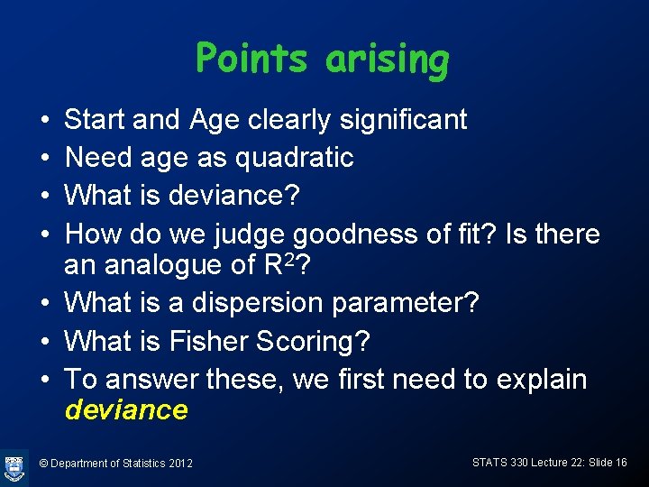
Points arising • • Start and Age clearly significant Need age as quadratic What is deviance? How do we judge goodness of fit? Is there an analogue of R 2? • What is a dispersion parameter? • What is Fisher Scoring? • To answer these, we first need to explain deviance © Department of Statistics 2012 STATS 330 Lecture 22: Slide 16

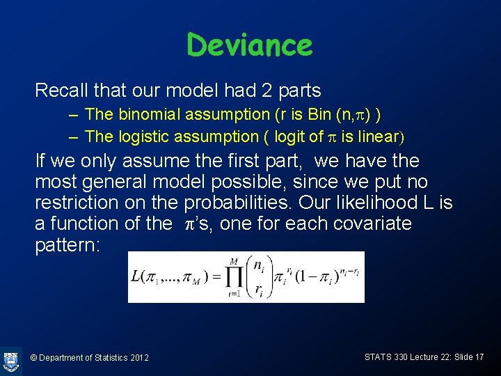
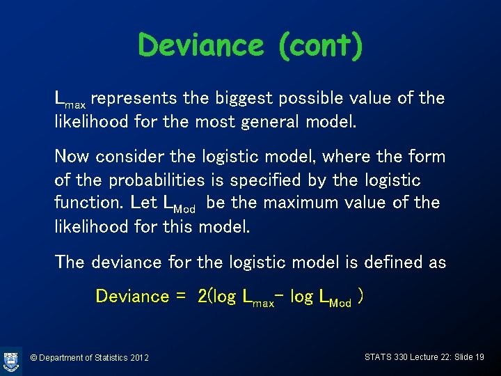
Deviance Recall that our model had 2 parts – The binomial assumption (r is Bin (n, p) ) – The logistic assumption ( logit of p is linear) If we only assume the first part, we have the most general model possible, since we put no restriction on the probabilities. Our likelihood L is a function of the p’s, one for each covariate pattern: © Department of Statistics 2012 STATS 330 Lecture 22: Slide 17

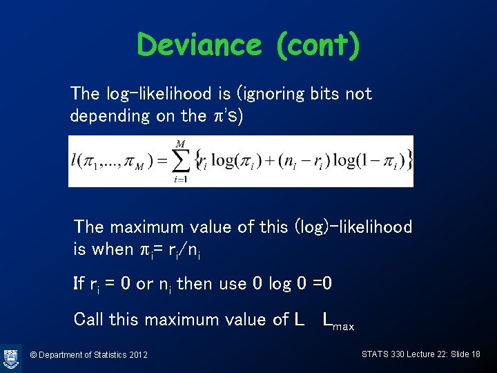
Deviance (cont) The log-likelihood is (ignoring bits not depending on the p’s) The maximum value of this (log)-likelihood is when pi= ri/ni If ri = 0 or ni then use 0 log 0 =0 Call this maximum value of L Lmax © Department of Statistics 2012 STATS 330 Lecture 22: Slide 18

Deviance (cont) Lmax represents the biggest possible value of the likelihood for the most general model. Now consider the logistic model, where the form of the probabilities is specified by the logistic function. Let LMod be the maximum value of the likelihood for this model. The deviance for the logistic model is defined as Deviance = 2(log Lmax- log LMod ) © Department of Statistics 2012 STATS 330 Lecture 22: Slide 19

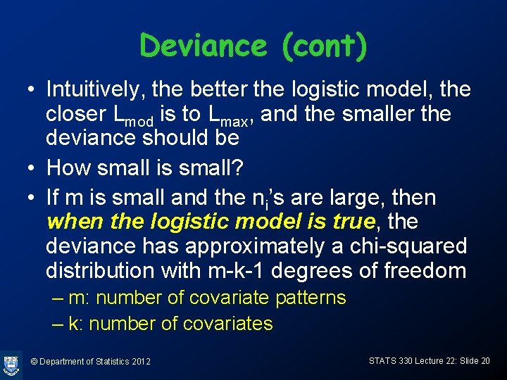
Deviance (cont) • Intuitively, the better the logistic model, the closer Lmod is to Lmax, and the smaller the deviance should be • How small is small? • If m is small and the ni’s are large, then when the logistic model is true, the deviance has approximately a chi-squared distribution with m-k-1 degrees of freedom – m: number of covariate patterns – k: number of covariates © Department of Statistics 2012 STATS 330 Lecture 22: Slide 20

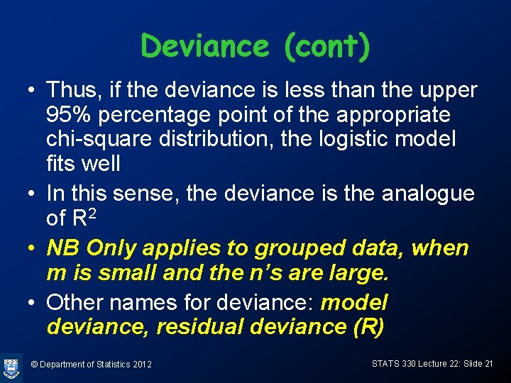
Deviance (cont) • Thus, if the deviance is less than the upper 95% percentage point of the appropriate chi-square distribution, the logistic model fits well • In this sense, the deviance is the analogue of R 2 • NB Only applies to grouped data, when m is small and the n’s are large. • Other names for deviance: model deviance, residual deviance (R) © Department of Statistics 2012 STATS 330 Lecture 22: Slide 21

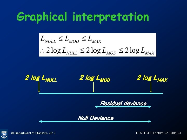
Null deviance • At the other extreme, the most restrictive model is one where all the probabilities pi are the same (ie don’t depend on the covariates). The deviance for this model is called the null deviance • Intuitively, if none of the covariates is related to the binary response, the model deviance won’t be much smaller then the null deviance © Department of Statistics 2012 STATS 330 Lecture 22: Slide 22

Graphical interpretation 2 log LNULL 2 log LMOD 2 log LMAX Residual deviance Null Deviance © Department of Statistics 2012 STATS 330 Lecture 22: Slide 23

Example: budworm data • Batches of 20 moths subjected to increasing doses of a poison, “success”=death • Data is grouped: for each of 6 doses (1. 0, 2. 0, 4. 0, 8. 0, 16. 0, 32. 0 mg) and each of male and female, we have 20 moths. • m=12 covariate patterns © Department of Statistics 2012 STATS 330 Lecture 22: Slide 24

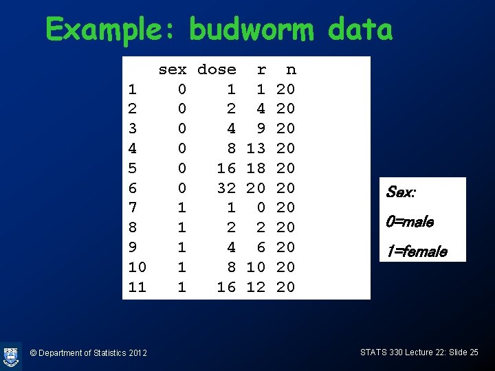
Example: budworm data sex dose r n 1 0 1 1 20 2 4 20 3 0 4 9 20 4 0 8 13 20 5 0 16 18 20 6 0 32 20 20 7 1 1 0 20 8 1 2 2 20 9 1 4 6 20 10 1 8 10 20 11 1 16 12 20 © Department of Statistics 2012 Sex: 0=male 1=female STATS 330 Lecture 22: Slide 25

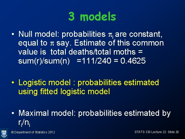
3 models • Null model: probabilities pi are constant, equal to p say. Estimate of this common value is total deaths/total moths = sum(r)/sum(n) =111/240 = 0. 4625 • Logistic model : probabilities estimated using fitted logistic model • Maximal model: probabilities estimated by ri/ni © Department of Statistics 2012 STATS 330 Lecture 22: Slide 26

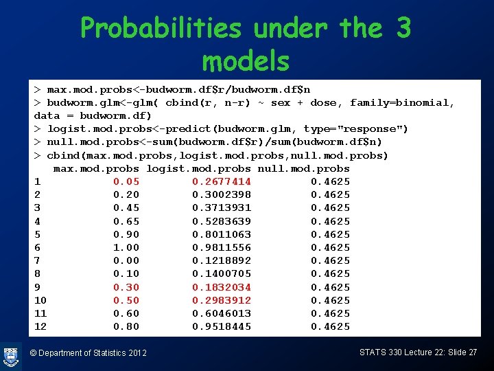
Probabilities under the 3 models > max. mod. probs<-budworm. df$r/budworm. df$n > budworm. glm<-glm( cbind(r, n-r) ~ sex + dose, family=binomial, data = budworm. df) > logist. mod. probs<-predict(budworm. glm, type="response") > null. mod. probs<-sum(budworm. df$r)/sum(budworm. df$n) > cbind(max. mod. probs, logist. mod. probs, null. mod. probs) max. mod. probs logist. mod. probs null. mod. probs 1 0. 05 0. 2677414 0. 4625 2 0. 20 0. 3002398 0. 4625 3 0. 45 0. 3713931 0. 4625 4 0. 65 0. 5283639 0. 4625 5 0. 90 0. 8011063 0. 4625 6 1. 00 0. 9811556 0. 4625 7 0. 00 0. 1218892 0. 4625 8 0. 10 0. 1400705 0. 4625 9 0. 30 0. 1832034 0. 4625 10 0. 50 0. 2983912 0. 4625 11 0. 6046013 0. 4625 12 0. 80 0. 9518445 0. 4625 © Department of Statistics 2012 STATS 330 Lecture 22: Slide 27

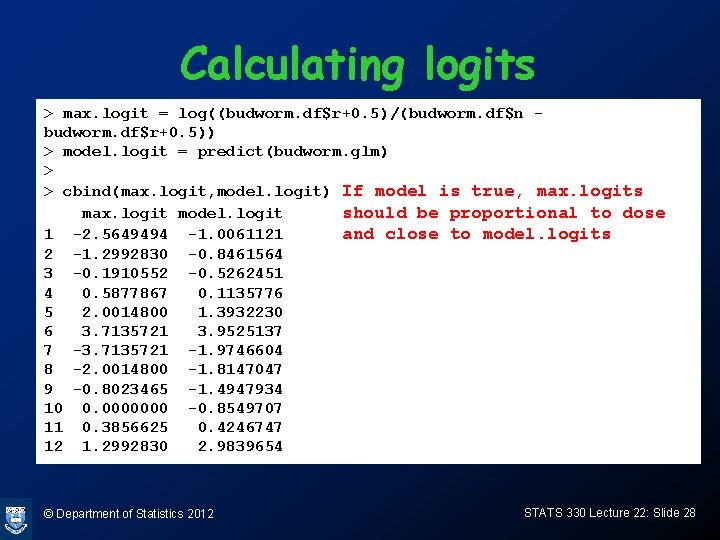
Calculating logits > max. logit = log((budworm. df$r+0. 5)/(budworm. df$n budworm. df$r+0. 5)) > model. logit = predict(budworm. glm) > > cbind(max. logit, model. logit) If model is true, max. logits max. logit model. logit should be proportional to dose 1 -2. 5649494 -1. 0061121 and close to model. logits 2 -1. 2992830 -0. 8461564 3 -0. 1910552 -0. 5262451 4 0. 5877867 0. 1135776 5 2. 0014800 1. 3932230 6 3. 7135721 3. 9525137 7 -3. 7135721 -1. 9746604 8 -2. 0014800 -1. 8147047 9 -0. 8023465 -1. 4947934 10 0. 0000000 -0. 8549707 11 0. 3856625 0. 4246747 12 1. 2992830 2. 9839654 © Department of Statistics 2012 STATS 330 Lecture 22: Slide 28

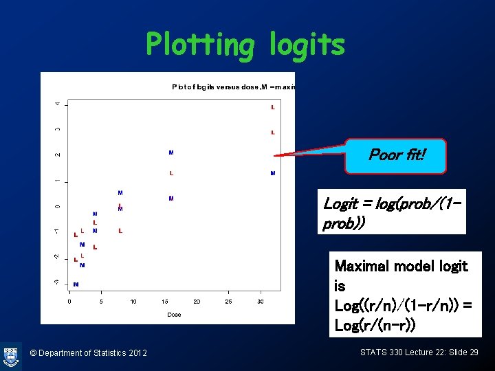
Plotting logits Poor fit! Logit = log(prob/(1 prob)) Maximal model logit is Log((r/n)/(1 -r/n)) = Log(r/(n-r)) © Department of Statistics 2012 STATS 330 Lecture 22: Slide 29

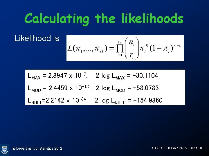
Calculating the likelihoods Likelihood is LMAX = 2. 8947 x 10 -7, 2 log LMAX = -30. 1104 LMOD = 2. 4459 x 10 -13 , 2 log LMOD = -58. 0783 LNULL=2. 2142 x 10 -34 , 2 log LNULL = -154. 9860 © Department of Statistics 2012 STATS 330 Lecture 22: Slide 30

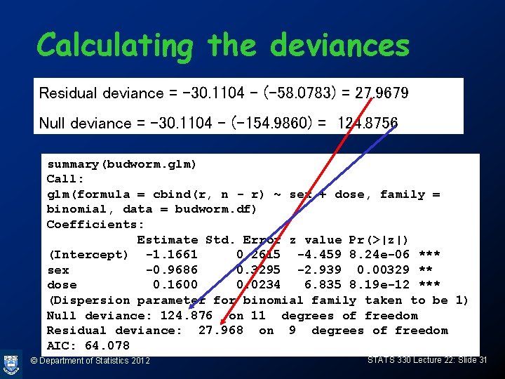
Calculating the deviances Residual deviance = -30. 1104 – (-58. 0783) = 27. 9679 Null deviance = -30. 1104 – (-154. 9860) = 124. 8756 summary(budworm. glm) Call: glm(formula = cbind(r, n - r) ~ sex + dose, family = binomial, data = budworm. df) Coefficients: Estimate Std. Error z value Pr(>|z|) (Intercept) -1. 1661 0. 2615 -4. 459 8. 24 e-06 *** sex -0. 9686 0. 3295 -2. 939 0. 00329 ** dose 0. 1600 0. 0234 6. 835 8. 19 e-12 *** (Dispersion parameter for binomial family taken to be 1) Null deviance: 124. 876 on 11 degrees of freedom Residual deviance: 27. 968 on 9 degrees of freedom AIC: 64. 078 © Department of Statistics 2012 STATS 330 Lecture 22: Slide 31

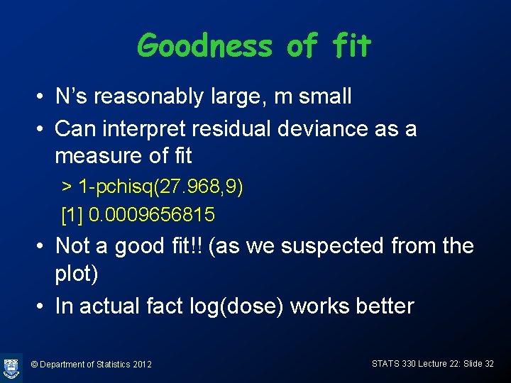
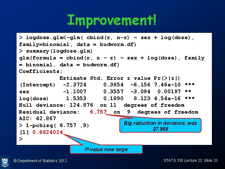
Goodness of fit • N’s reasonably large, m small • Can interpret residual deviance as a measure of fit > 1 -pchisq(27. 968, 9) [1] 0. 0009656815 • Not a good fit!! (as we suspected from the plot) • In actual fact log(dose) works better © Department of Statistics 2012 STATS 330 Lecture 22: Slide 32

Improvement! > logdose. glm<-glm( cbind(r, n-r) ~ sex + log(dose), family=binomial, data = budworm. df) > summary(logdose. glm) glm(formula = cbind(r, n - r) ~ sex + log(dose), family = binomial, data = budworm. df) Coefficients: Estimate Std. Error z value Pr(>|z|) (Intercept) -2. 3724 0. 3854 -6. 156 7. 46 e-10 *** sex -1. 1007 0. 3557 -3. 094 0. 00197 ** log(dose) 1. 5353 0. 1890 8. 123 4. 54 e-16 *** Null deviance: 124. 876 on 11 degrees of freedom Residual deviance: 6. 757 on 9 degrees of freedom AIC: 42. 867 Big reduction in deviance, was > 1 -pchisq( 6. 757 , 9) 27. 968 [1] 0. 6624024 > P-value now large © Department of Statistics 2012 STATS 330 Lecture 22: Slide 33