Statistics The POWER of Data Statistics Definition Statistics

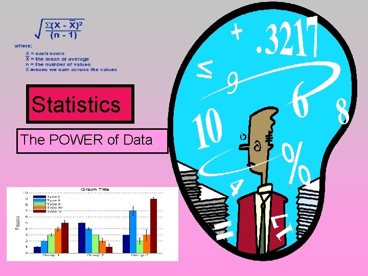
Statistics The POWER of Data

Statistics: Definition Statistics is the mathematics of the collection, organization, and interpretation of numerical data.

Data • Data is information, in the form of facts or figures, used as a basis for making calculations or drawing conclusions • Data can be quantitative or qualitative. • Data can be obtained by a variety of methodologies: – Random Sample – Quadrat Study – Questionnaires – Experiments

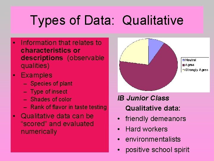
Types of Data: Qualitative • Information that relates to characteristics or descriptions (observable qualities) • Examples – – Species of plant Type of insect Shades of color Rank of flavor in taste testing • Qualitative data can be “scored” and evaluated numerically IB Junior Class Qualitative data: • friendly demeanors • Hard workers • environmentalists • positive school spirit

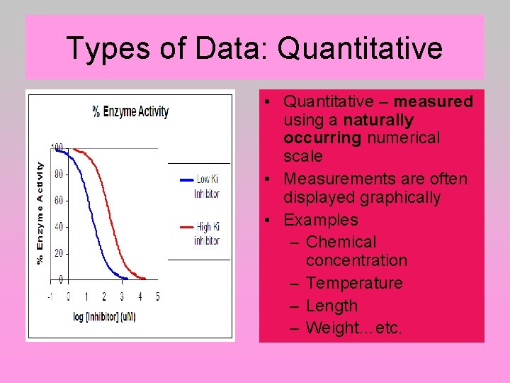
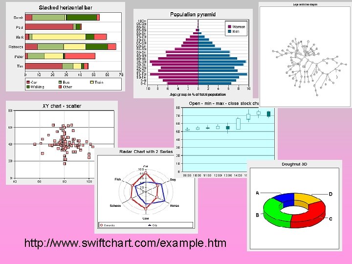
Types of Data: Quantitative • Quantitative – measured using a naturally occurring numerical scale • Measurements are often displayed graphically • Examples – Chemical concentration – Temperature – Length – Weight…etc.

http: //www. swiftchart. com/example. htm

Error Analysis • ALL measurements are subject to uncertainties and this must always be stated. – Measure someone’s height. Are they slouching? Wearing shoes? Standing on even ground? Is it morning or night? – Measuring multiple times REDUCES the error!! • • The limits of the equipment used add some uncertainty to the data collected. All equipment has a certain magnitude of uncertainty. For example, is a ruler that is massproduced a good measure of 1 cm? 1 mm? 0. 1 mm? For quantitative testing, you must indicate the level of uncertainty of the tool that you are using for measurement!!

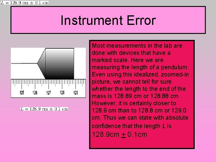
Instrument Error Most measurements in the lab are done with devices that have a marked scale. Here we are measuring the length of a pendulum. Even using this idealized, zoomed-in picture, we cannot tell for sure whether the length to the end of the mass is 128. 89 cm or 128. 88 cm. However, it is certainly closer to 128. 9 cm than to 128. 8 cm or 129. 0 cm. Thus we can state with absolute confidence that the length L is 128. 9 cm + 0. 1 cm

Error and Electronics • ALL devices have an error potential; sometimes it is written on the instrument itself • The error of an electronic device is usually half of the last precision digit.

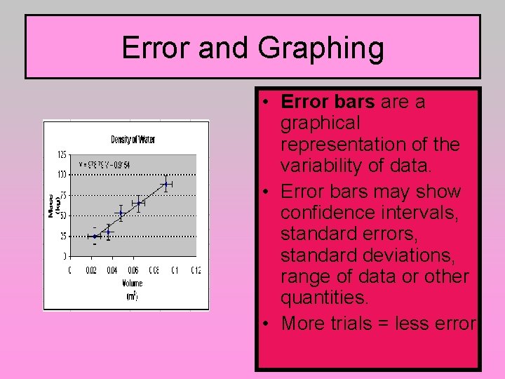
Error and Graphing • Error bars are a graphical representation of the variability of data. • Error bars may show confidence intervals, standard errors, standard deviations, range of data or other quantities. • More trials = less error

Significant Figures • Be sure that the number of significant digits in the data table/graph reflects the precision of the instrument used (for ex. If the manufacturer states that the accuracy of a balance is to 0. 1 g – and your average mass is 2. 06 g, be sure to round the average to 2. 1 g) Your data must be consistent with your measurement tool regarding significant figures.

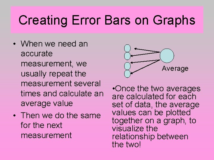
Creating Error Bars on Graphs • When we need an accurate measurement, we usually repeat the measurement several times and calculate an average value • Then we do the same for the next measurement Average • Once the two averages are calculated for each set of data, the average values can be plotted together on a graph, to visualize the relationship between the two!

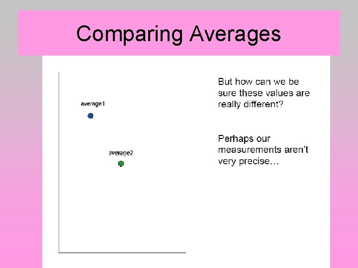
Comparing Averages

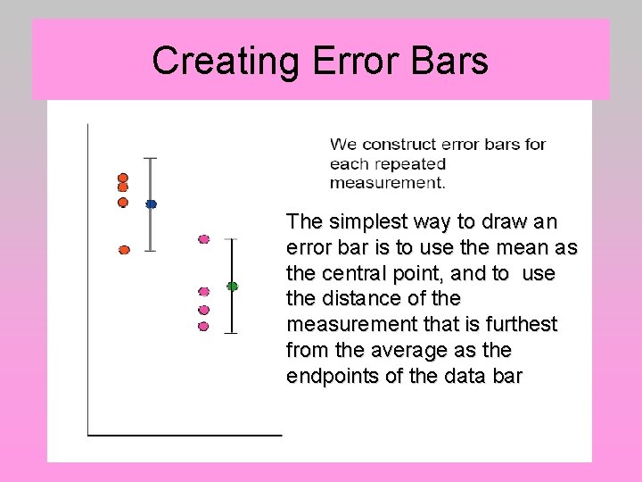
Creating Error Bars The simplest way to draw an error bar is to use the mean as the central point, and to use the distance of the measurement that is furthest from the average as the endpoints of the data bar

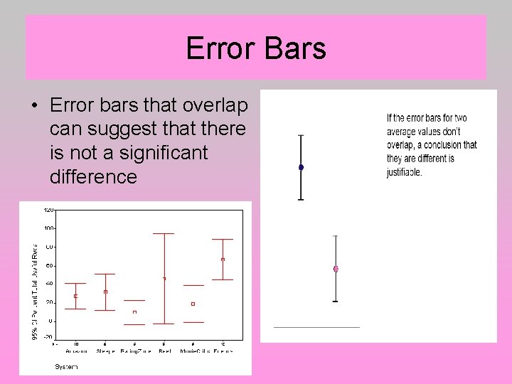
Error Bars • Error bars that overlap can suggest that there is not a significant difference

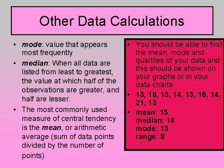
Other Data Calculations • mode: value that appears most frequently • median: When all data are listed from least to greatest, the value at which half of the observations are greater, and half are lesser. • The most commonly used measure of central tendency is the mean, or arithmetic average (sum of data points divided by the number of points) • You should be able to find the mean, mode and quartiles of your data and this should be shown on your graphs or in your data charts. • 13, 18, 13, 14, 13, 16, 14, 21, 13 • mean: 15 median: 14 mode: 13 range: 8

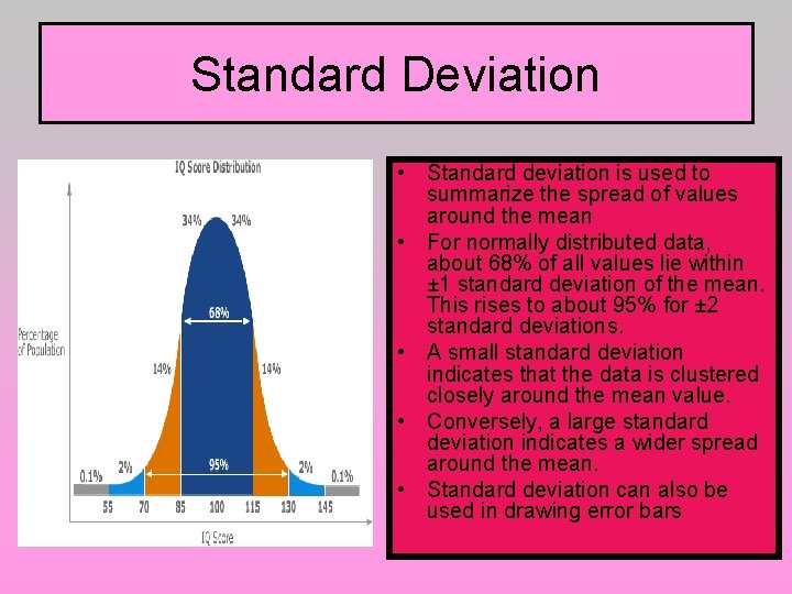
Standard Deviation • Standard deviation is used to summarize the spread of values around the mean • For normally distributed data, about 68% of all values lie within ± 1 standard deviation of the mean. This rises to about 95% for ± 2 standard deviations. • A small standard deviation indicates that the data is clustered closely around the mean value. • Conversely, a large standard deviation indicates a wider spread around the mean. • Standard deviation can also be used in drawing error bars

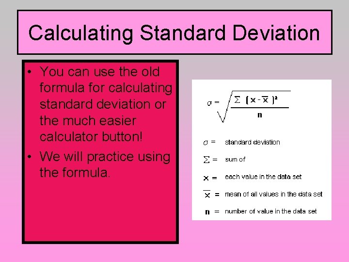
Calculating Standard Deviation • You can use the old formula for calculating standard deviation or the much easier calculator button! • We will practice using the formula.

Calculating Standard Deviation • Standard Deviation can be calculated: – on your calculator – In Microsoft excel (type the following code into the cell where you want the standard deviation result, using the “unbiased, ” or “n 1” method: STDEV(A 1: A 30) (substitute the cell name of the first value in your dataset for A 1, and the cell name of the last value for A 30. ) – On your computer: http: //www. pages. drexel. ed u/~jdf 37/mean. htm

Let’s measure some people!!

Is our data reliable enough to support a conclusion?

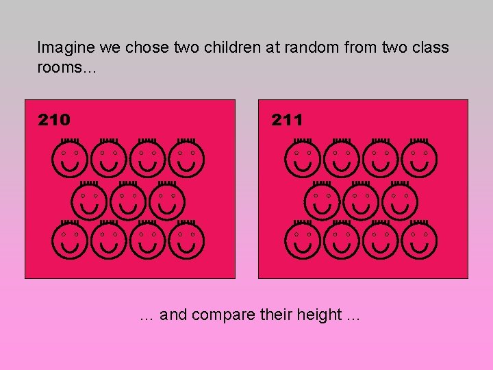
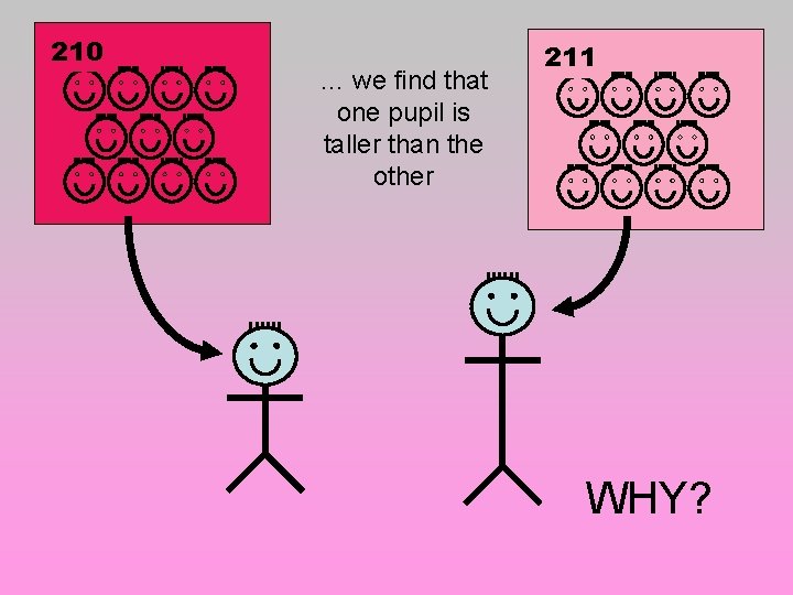
Imagine we chose two children at random from two class rooms… 210 211 … and compare their height …

210 … we find that one pupil is taller than the other 211 WHY?

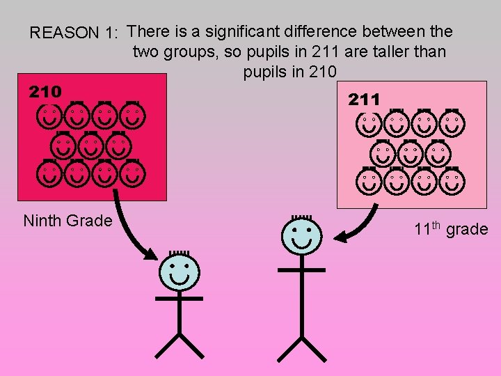
REASON 1: There is a significant difference between the two groups, so pupils in 211 are taller than pupils in 210 211 Ninth Grade 11 th grade

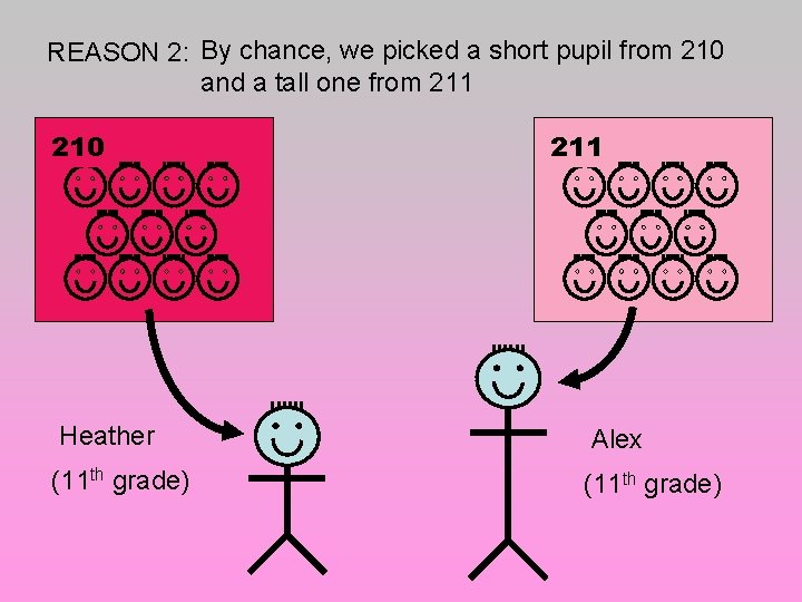
REASON 2: By chance, we picked a short pupil from 210 and a tall one from 211 210 211 Heather Alex (11 th grade)

How do we decide which reason is most likely? MEASURE MORE STUDENTS!!!

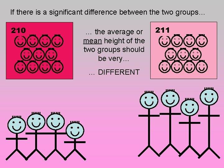
If there is a significant difference between the two groups… 210 … the average or mean height of the two groups should be very… … DIFFERENT 211

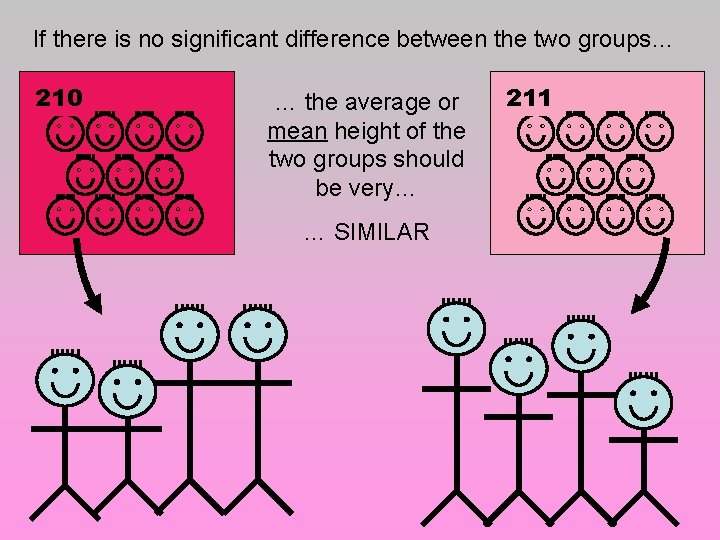
If there is no significant difference between the two groups… 210 … the average or mean height of the two groups should be very… … SIMILAR 211

Remember: Living things normally show a lot of variation, so…

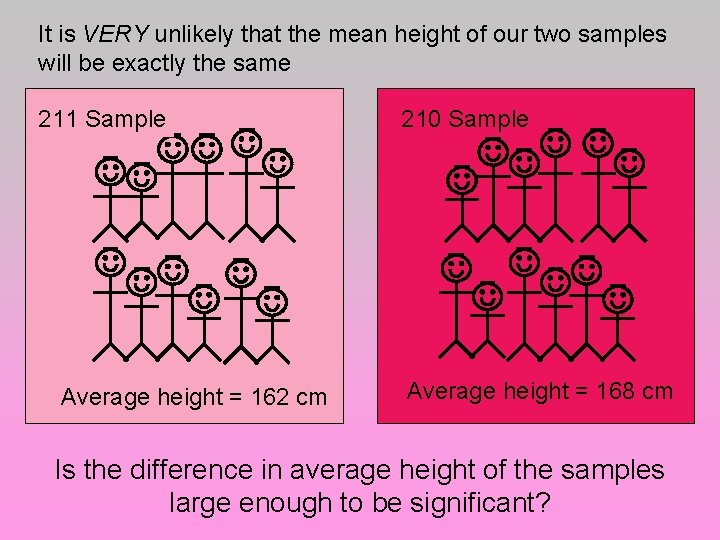
It is VERY unlikely that the mean height of our two samples will be exactly the same 211 Sample Average height = 162 cm 210 Sample Average height = 168 cm Is the difference in average height of the samples large enough to be significant?

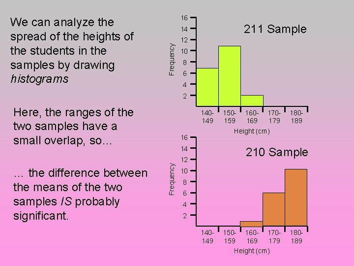
16 211 Sample 14 Frequency We can analyze the spread of the heights of the students in the samples by drawing histograms 12 10 8 6 4 2 Here, the ranges of the two samples have a small overlap, so… 16 14 Frequency … the difference between the means of the two samples IS probably significant. 140149 150 - 160 - 170159 169 179 Height (cm) 180189 210 Sample 12 10 8 6 4 2 140149 150 - 160 - 170159 169 179 Height (cm) 180189

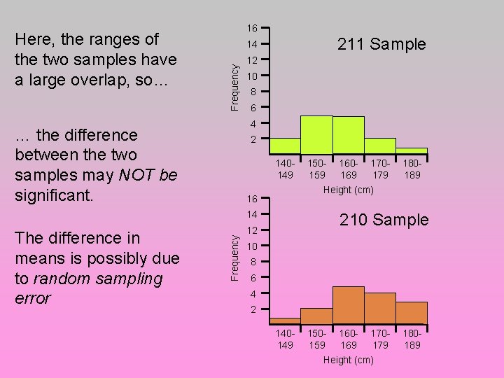
211 Sample 14 Frequency Here, the ranges of the two samples have a large overlap, so… 16 12 10 8 6 4 … the difference between the two samples may NOT be significant. 2 140149 16 The difference in means is possibly due to random sampling error Frequency 14 150 - 160 - 170159 169 179 Height (cm) 180189 210 Sample 12 10 8 6 4 2 140149 150 - 160 - 170159 169 179 Height (cm) 180189

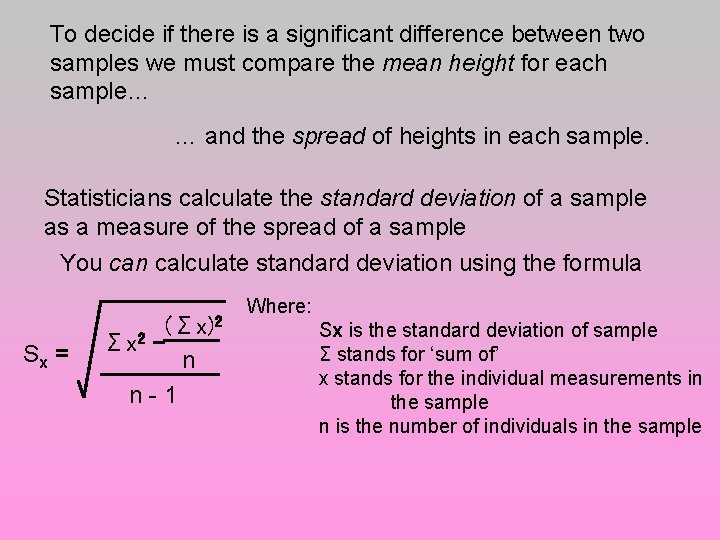
To decide if there is a significant difference between two samples we must compare the mean height for each sample… … and the spread of heights in each sample. Statisticians calculate the standard deviation of a sample as a measure of the spread of a sample You can calculate standard deviation using the formula Sx = Σx 2 - (Σx)2 n-1 n Where: Sx is the standard deviation of sample Σ stands for ‘sum of’ x stands for the individual measurements in the sample n is the number of individuals in the sample

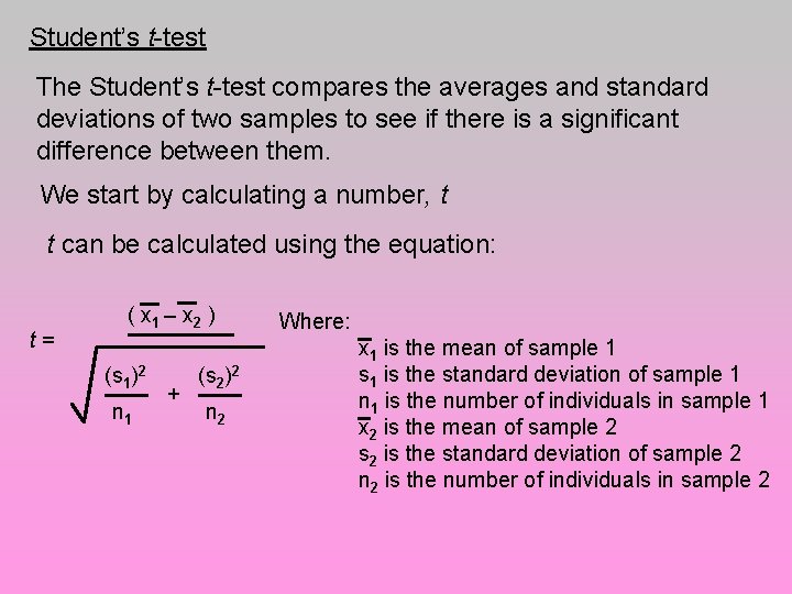
Student’s t-test The Student’s t-test compares the averages and standard deviations of two samples to see if there is a significant difference between them. We start by calculating a number, t t can be calculated using the equation: t= ( x 1 – x 2 ) (s 1)2 n 1 + (s 2)2 n 2 Where: x 1 is the mean of sample 1 s 1 is the standard deviation of sample 1 n 1 is the number of individuals in sample 1 x 2 is the mean of sample 2 s 2 is the standard deviation of sample 2 n 2 is the number of individuals in sample 2

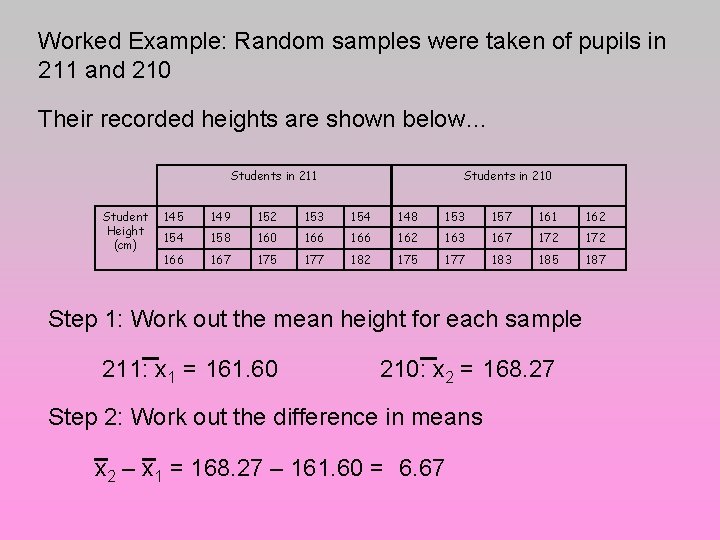
Worked Example: Random samples were taken of pupils in 211 and 210 Their recorded heights are shown below… Students in 211 Student Height (cm) Students in 210 145 149 152 153 154 148 153 157 161 162 154 158 160 166 162 163 167 172 166 167 175 177 182 175 177 183 185 187 Step 1: Work out the mean height for each sample 211: x 1 = 161. 60 210: x 2 = 168. 27 Step 2: Work out the difference in means x 2 – x 1 = 168. 27 – 161. 60 = 6. 67

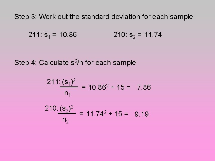
Step 3: Work out the standard deviation for each sample 211: s 1 = 10. 86 210: s 2 = 11. 74 Step 4: Calculate s 2/n for each sample 211: (s 1)2 n 1 210: (s 2)2 n 2 = 10. 862 ÷ 15 = 7. 86 = 11. 742 ÷ 15 = 9. 19

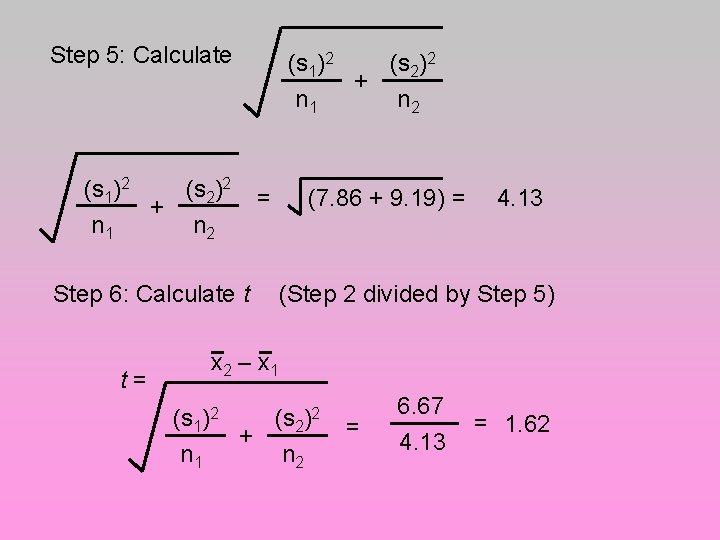
Step 5: Calculate (s 1)2 n 1 + (s 2)2 = + (s 2)2 n 2 (7. 86 + 9. 19) = 4. 13 n 2 Step 6: Calculate t (Step 2 divided by Step 5) x 2 – x 1 t= (s 1)2 n 1 + (s 2)2 n 2 = 6. 67 4. 13 = 1. 62

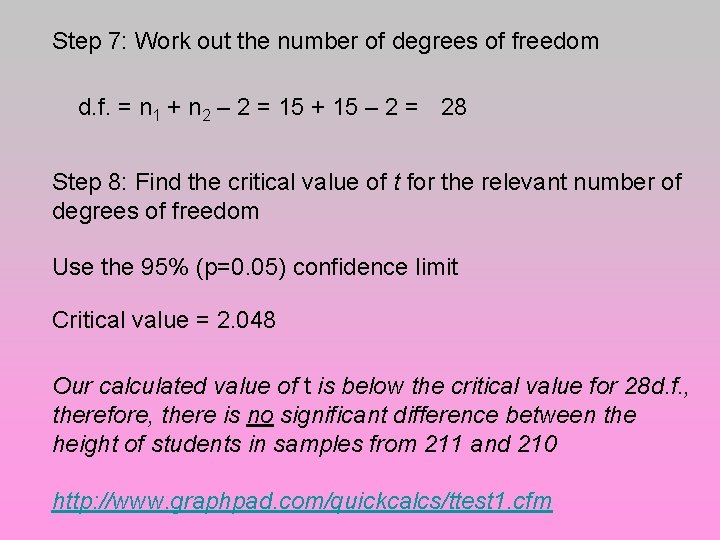
Step 7: Work out the number of degrees of freedom d. f. = n 1 + n 2 – 2 = 15 + 15 – 2 = 28 Step 8: Find the critical value of t for the relevant number of degrees of freedom Use the 95% (p=0. 05) confidence limit Critical value = 2. 048 Our calculated value of t is below the critical value for 28 d. f. , therefore, there is no significant difference between the height of students in samples from 211 and 210 http: //www. graphpad. com/quickcalcs/ttest 1. cfm

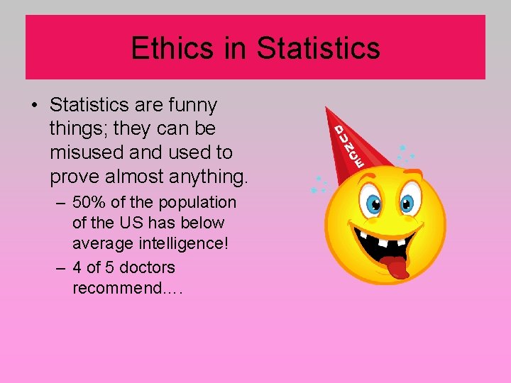
Ethics in Statistics • Statistics are funny things; they can be misused and used to prove almost anything. – 50% of the population of the US has below average intelligence! – 4 of 5 doctors recommend….

Ways of Misusing Data • Recreate experiment until the numbers say what you want. (interview MANY groups of 5 dentists) • NEVER IGNORE DATA THAT DOESN’T SEEM TO MATCH YOUR BELIEFS!!!!!

Misusing Data: Dos and Don’ts • The amount of data matters! More data is more reliable • Avoid bias! Don’t have a perceived idea of what will happen (this is hard!) • Accidents occur! 5% of results are likely to happen by accident (False alarm probability) • Don’t discard some data; all data is important even if unexpected. • Don’t over generalize (All apples are red) • Don’t manipulate • Don’t make up “better” data

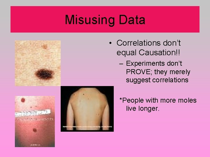
Misusing Data • Correlations don’t equal Causation!! – Experiments don’t PROVE; they merely suggest correlations *People with more moles live longer.

Data Misuse Examples • Bell Curve – There are substantial individual and group differences in intelligence; these differences profoundly influence the social structure and organization of work in modern industrial societies, and they defy easy remediation.

FREAKONOMICS • Schoolteachers and Sumo wrestlers have a lot in common. • The Ku Klux Klan and Real Estate Agents work under the same principles • Abortion lessons crime! • Do names matter? – Low education parents: Ricky, Terry, Larry, Jazmine, Misty, Mercedes – High education parents: Marie-Claire, Glynnis, Aviva, Finnegan, Mac. Gregor, Harper – ? ? ? : Loser, Winner, Temptress, Sir John, Precious