Statistics review of basic probability and statistics Statistics

Statistics review of basic probability and statistics

Statistics • Outline –Introduction –Random Variables –Simulation Output 040669 || WS 2008 || Dr. Verena Schmid || PR KFK PM/SCM/TL Praktikum Simulation I 2

Statistics • integral part of simulation studys –model probabilistic systems –validate simulation model –choose input probability distributions –generate random samples –perform statistical analysis 040669 || WS 2008 || Dr. Verena Schmid || PR KFK PM/SCM/TL Praktikum Simulation I 3

density and distribution functions Random Variables 040669 || WS 2008 || Dr. Verena Schmid || PR KFK PM/SCM/TL Praktikum Simulation I 4

Experiments • experiment –process whose output is not known with certainty –sample space (S): set of all possible outcomes –sample points: outcomes in the sample space • examples: –flipping a coin: S = {H, T} –toss a die: S = {1, 2, 3, 4, 5, 6} • random variable –assigns a real number to each point in the sample space 040669 || WS 2008 || Dr. Verena Schmid || PR KFK PM/SCM/TL Praktikum Simulation I 5

Random Variable • discrete random variables –a random variable X is said to be discrete if it can take on at most a countable number of values x 1, x 2, x 3, . . , xn –probability mass function: the probability that X takes on the value xi is given by –probability that X lies in Interval I [a, b] –(cumulative) distribution function 040669 || WS 2008 || Dr. Verena Schmid || PR KFK PM/SCM/TL Praktikum Simulation I 6

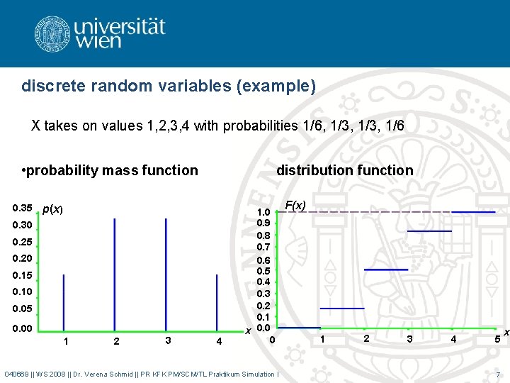
discrete random variables (example) X takes on values 1, 2, 3, 4 with probabilities 1/6, 1/3, 1/6 • probability mass function 0. 35 distribution function p(x) 0. 30 0. 25 0. 20 0. 15 0. 10 0. 05 0. 00 1 2 3 4 1. 0 0. 9 0. 8 0. 7 0. 6 0. 5 0. 4 0. 3 0. 2 0. 1 x 0. 0 0 040669 || WS 2008 || Dr. Verena Schmid || PR KFK PM/SCM/TL Praktikum Simulation I F(x) 1 2 3 4 5 7 x

Random Variable (cont. ) • continuous random variables –a random variable X is said to be continuous if it can take on an uncountable infinite number of different values –probability density function: nonnegative function • for any set of real numbers B (ex. B = [1, 2]) • its not the probability a continuous random variable X equals x • different interpretation (for ¢x > 0) 040669 || WS 2008 || Dr. Verena Schmid || PR KFK PM/SCM/TL Praktikum Simulation I 8

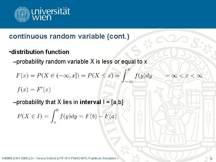
continuous random variable (cont. ) • distribution function –probability random variable X is less or equal to x –probability that X lies in interval I = [a, b] 040669 || WS 2008 || Dr. Verena Schmid || PR KFK PM/SCM/TL Praktikum Simulation I 9

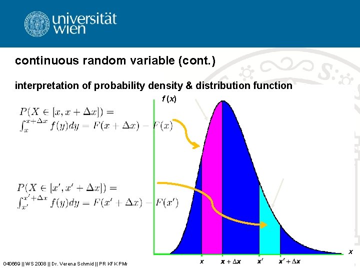
continuous random variable (cont. ) interpretation of probability density & distribution function f (x) x 040669 || WS 2008 || Dr. Verena Schmid || PR KFK PM/SCM/TL Praktikum Simulation I 10

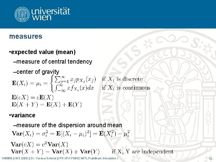
measures • expected value (mean) –measure of central tendency –center of gravity • variance –measure of the dispersion around mean 040669 || WS 2008 || Dr. Verena Schmid || PR KFK PM/SCM/TL Praktikum Simulation I 12

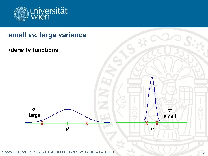
small vs. large variance • density functions σ2 large σ2 small X µ X 040669 || WS 2008 || Dr. Verena Schmid || PR KFK PM/SCM/TL Praktikum Simulation I X µ X 13

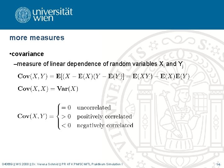
more measures • covariance –measure of linear dependence of random variables Xi and Yj 040669 || WS 2008 || Dr. Verena Schmid || PR KFK PM/SCM/TL Praktikum Simulation I 14

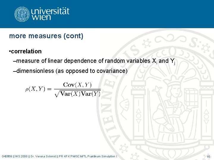
more measures (cont) • correlation –measure of linear dependence of random variables Xi and Yj –dimensionless (as opposed to covariance) 040669 || WS 2008 || Dr. Verena Schmid || PR KFK PM/SCM/TL Praktikum Simulation I 15

example distributions 040669 || WS 2008 || Dr. Verena Schmid || PR KFK PM/SCM/TL Praktikum Simulation I 16

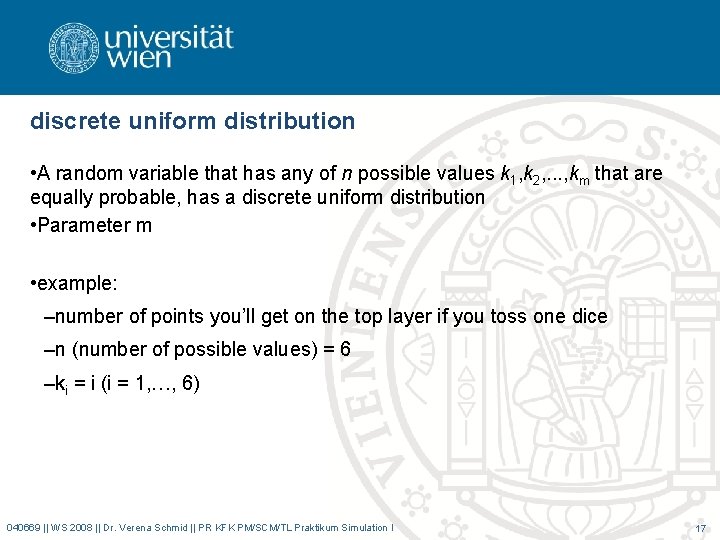
discrete uniform distribution • A random variable that has any of n possible values k 1, k 2, . . . , km that are equally probable, has a discrete uniform distribution • Parameter m • example: –number of points you’ll get on the top layer if you toss one dice –n (number of possible values) = 6 –ki = i (i = 1, …, 6) 040669 || WS 2008 || Dr. Verena Schmid || PR KFK PM/SCM/TL Praktikum Simulation I 17

binomial distribution A typical example is the following: assume 5% of the population is HIVpositive. You pick 500 people randomly. How likely is it that you get 30 or more HIV-positives? –Parameters n and p 040669 || WS 2008 || Dr. Verena Schmid || PR KFK PM/SCM/TL Praktikum Simulation I 18

normal distribution N(m, s) • probability density function f(x) also called Gaussian distribution - extremely important probability distribution in many fields • distribution function F(x) 040669 || WS 2008 || Dr. Verena Schmid || PR KFK PM/SCM/TL Praktikum Simulation I 19

poisson distribution • Distribution of “rare” events –Parameters l • usually used for modeling number of arrivals per time unit 040669 || WS 2008 || Dr. Verena Schmid || PR KFK PM/SCM/TL Praktikum Simulation I 20

geometric distribution For example, suppose an ordinary die is thrown repeatedly until the first time a "1" appears. The probability distribution of the number of times it is thrown is supported on the infinite set { 1, 2, 3, . . . } and is a geometric distribution with p = 1/6. –Parameter p 040669 || WS 2008 || Dr. Verena Schmid || PR KFK PM/SCM/TL Praktikum Simulation I 21

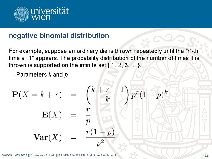
negative binomial distribution For example, suppose an ordinary die is thrown repeatedly until the “r”-th time a "1" appears. The probability distribution of the number of times it is thrown is supported on the infinite set { 1, 2, 3, . . . }. –Parameters k and p 040669 || WS 2008 || Dr. Verena Schmid || PR KFK PM/SCM/TL Praktikum Simulation I 22

hypergeometric distribution • A typical example is the following: There is a shipment of N objects in which M are defective. The hypergeometric distribution describes the probability that in a sample of n distinctive objects drawn from the shipment exactly k objects are defective. –Parameters N, M, and n 040669 || WS 2008 || Dr. Verena Schmid || PR KFK PM/SCM/TL Praktikum Simulation I 23

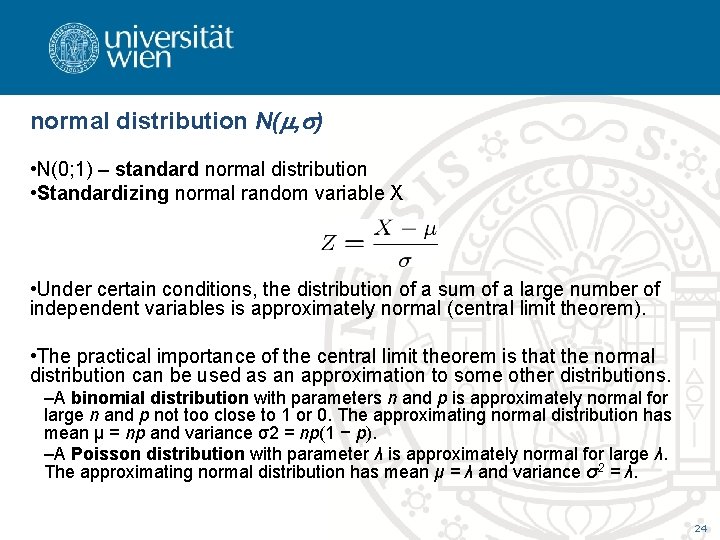
normal distribution N(m, s) • N(0; 1) – standard normal distribution • Standardizing normal random variable X • Under certain conditions, the distribution of a sum of a large number of independent variables is approximately normal (central limit theorem). • The practical importance of the central limit theorem is that the normal distribution can be used as an approximation to some other distributions. –A binomial distribution with parameters n and p is approximately normal for large n and p not too close to 1 or 0. The approximating normal distribution has mean μ = np and variance σ2 = np(1 − p). –A Poisson distribution with parameter λ is approximately normal for large λ. The approximating normal distribution has mean μ = λ and variance σ2 = λ. 24

uniform distribution • probability density function f(x) each result in interval [0, 1] has the 1 same probability 0 1 • distribution function F(x) 040669 || WS 2008 || Dr. Verena Schmid || PR KFK PM/SCM/TL Praktikum Simulation I 25

uniform distribution • probability density function f(x) each result in interval [a, b] has the same probability • distribution function F(x) 040669 || WS 2008 || Dr. Verena Schmid || PR KFK PM/SCM/TL Praktikum Simulation I 26

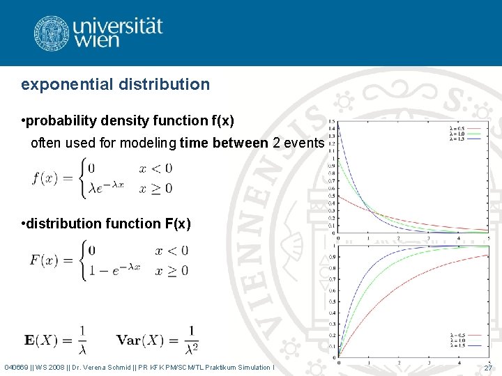
exponential distribution • probability density function f(x) often used for modeling time between 2 events • distribution function F(x) 040669 || WS 2008 || Dr. Verena Schmid || PR KFK PM/SCM/TL Praktikum Simulation I 27

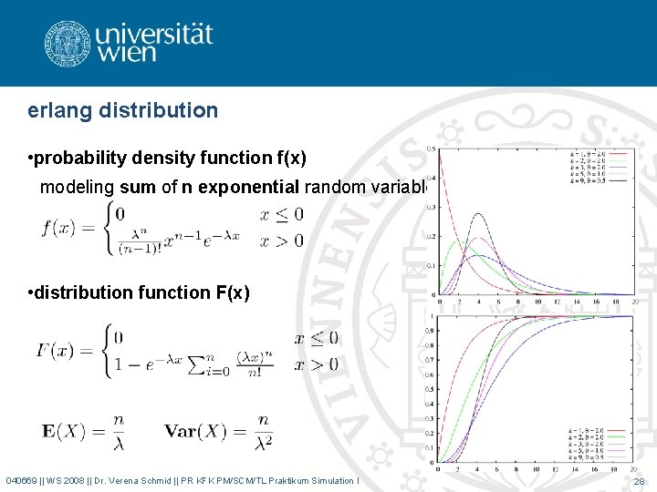
erlang distribution • probability density function f(x) modeling sum of n exponential random variables • distribution function F(x) 040669 || WS 2008 || Dr. Verena Schmid || PR KFK PM/SCM/TL Praktikum Simulation I 28

Estimation 040669 || WS 2008 || Dr. Verena Schmid || PR KFK PM/SCM/TL Praktikum Simulation I 29

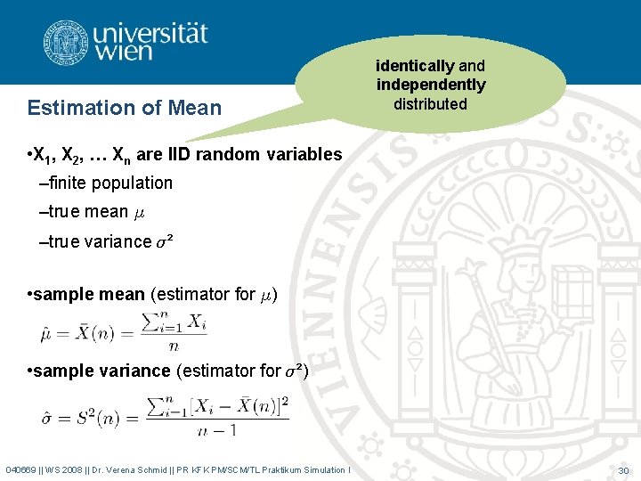
Estimation of Mean identically and independently distributed • X 1, X 2, … Xn are IID random variables –finite population –true mean ¹ –true variance ¾² • sample mean (estimator for ¹) • sample variance (estimator for ¾²) 040669 || WS 2008 || Dr. Verena Schmid || PR KFK PM/SCM/TL Praktikum Simulation I 30

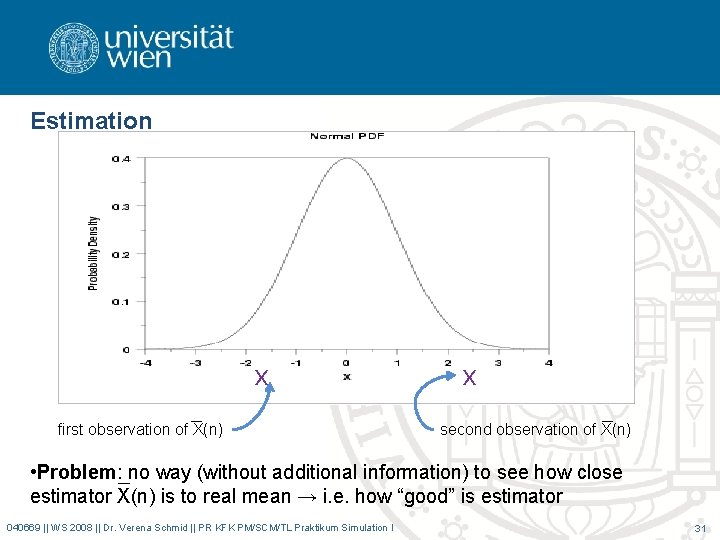
Estimation x first observation of X(n) x second observation of X(n) • Problem: no way (without additional information) to see how close estimator X(n) is to real mean → i. e. how “good” is estimator 040669 || WS 2008 || Dr. Verena Schmid || PR KFK PM/SCM/TL Praktikum Simulation I 31

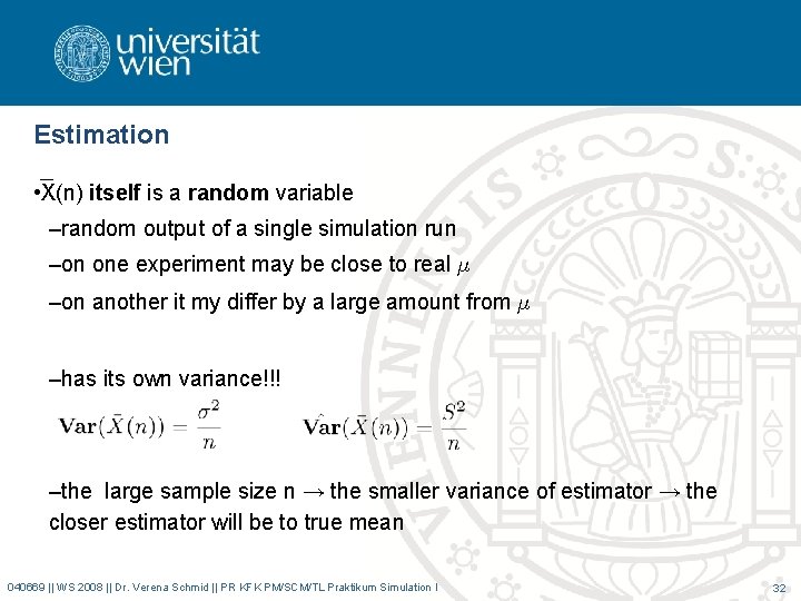
Estimation • X(n) itself is a random variable –random output of a single simulation run –on one experiment may be close to real ¹ –on another it my differ by a large amount from ¹ –has its own variance!!! –the large sample size n → the smaller variance of estimator → the closer estimator will be to true mean 040669 || WS 2008 || Dr. Verena Schmid || PR KFK PM/SCM/TL Praktikum Simulation I 32

Estimation: construct confidence interval central limit theorem says… for large sample size n the estimator (sample mean) X(n) is approximately normally distributed with mean ¹ and variance ¾²/n problem real variance ¾² is usually unknown (but sample variance S²(n) converges to ¾² as n is “large enough”) 040669 || WS 2008 || Dr. Verena Schmid || PR KFK PM/SCM/TL Praktikum Simulation I 33

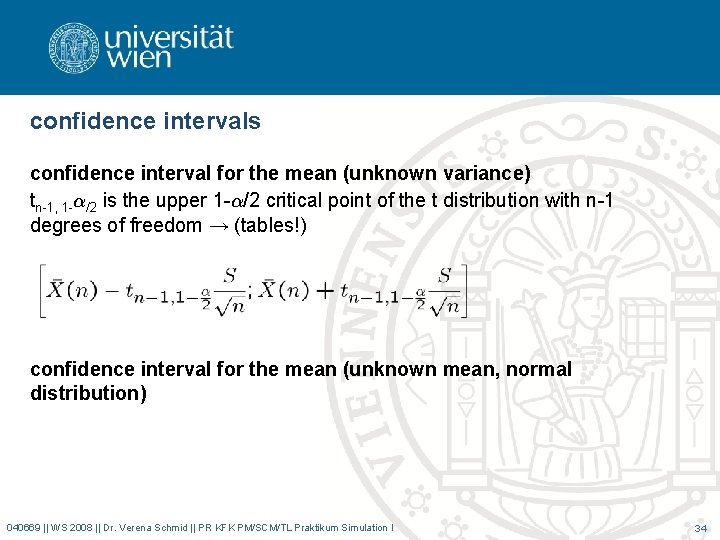
confidence intervals confidence interval for the mean (unknown variance) tn-1, 1 -®/2 is the upper 1 -®/2 critical point of the t distribution with n-1 degrees of freedom → (tables!) confidence interval for the mean (unknown mean, normal distribution) 040669 || WS 2008 || Dr. Verena Schmid || PR KFK PM/SCM/TL Praktikum Simulation I 34

confidence intervals interpretation: nothing probabilistic about confidence intervals (once they have been created – just numbers) if one constructs a very large number of independent confidence intervals, each based on n (“sufficiently large”) observations, the proportion of these confidence intervals that cover the real ¹ is equal to 1 -® 040669 || WS 2008 || Dr. Verena Schmid || PR KFK PM/SCM/TL Praktikum Simulation I 35

example: confidence intervals 10 observations 1. 2 1. 5 1. 68 1. 89 0. 95 1. 49 1. 58 1. 55 0. 5 1. 09 sample size n = 10 estimator for mean X(10) = 1. 343 estimator for variance S²(10) = 0. 16751222 90% confidence interval (® = 10%) 040669 || WS 2008 || Dr. Verena Schmid || PR KFK PM/SCM/TL Praktikum Simulation I 36

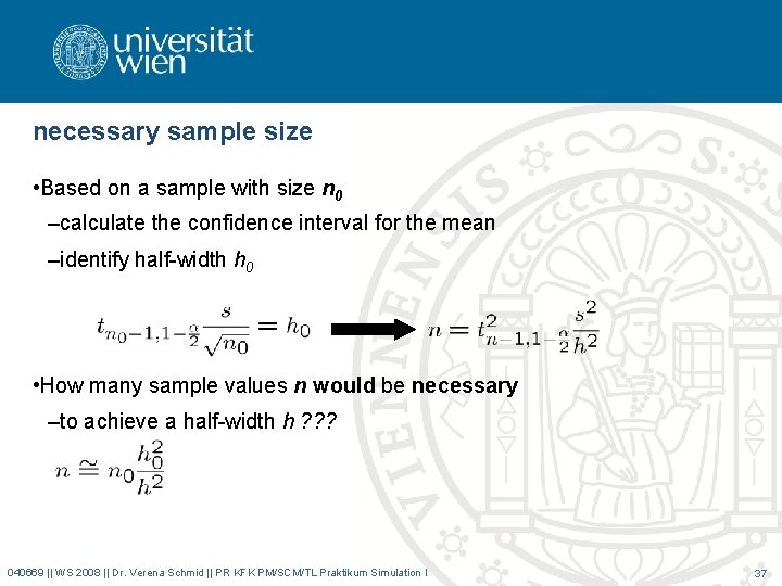
necessary sample size • Based on a sample with size n 0 –calculate the confidence interval for the mean –identify half-width h 0 • How many sample values n would be necessary –to achieve a half-width h ? ? ? 040669 || WS 2008 || Dr. Verena Schmid || PR KFK PM/SCM/TL Praktikum Simulation I 37

example (cont) 10 observations 1. 2 1. 5 1. 68 1. 89 0. 95 1. 49 1. 58 1. 55 0. 5 1. 09 • based on n 0 = 10 observations –half width h 0 = 0. 24 Q: if you’d prefer a half width of 0. 12 –what’s the necessary number of observation? ? 040669 || WS 2008 || Dr. Verena Schmid || PR KFK PM/SCM/TL Praktikum Simulation I 38

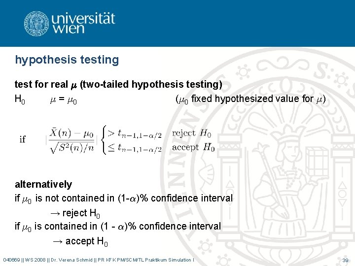
hypothesis testing test for real ¹ (two-tailed hypothesis testing) H 0 ¹ = ¹ 0 (¹ 0 fixed hypothesized value for ¹) alternatively if ¹ 0 is not contained in (1 -®)% confidence interval → reject H 0 if ¹ 0 is contained in (1 - ®)% confidence interval → accept H 0 040669 || WS 2008 || Dr. Verena Schmid || PR KFK PM/SCM/TL Praktikum Simulation I 39

Comparison of 2 Alternatives • Confidence Intervals for the difference of the means (independent) –equal variances, but unknown –different variances 040669 || WS 2008 || Dr. Verena Schmid || PR KFK PM/SCM/TL Praktikum Simulation I 40