Statistics Review Levels of Measurement Levels of Measurement

Statistics Review Levels of Measurement

Levels of Measurement Nominal scale • Nominal measurement consists of assigning items to groups or categories. • No quantitative information is conveyed and no ordering of the items is implied. • Nominal scales are therefore qualitative rather than quantitative. • Examples: Religious preference, race, and gender are all examples of nominal scales • Statistics: Sum, Frequency Distributions

Ordinal Scale • Measurements with ordinal scales are ordered: higher numbers represent higher values. • However, the intervals between the numbers are not necessarily equal. • There is no "true" zero point for ordinal scales since the zero point is chosen arbitrarily. • For example, on a five-point Likert scale, the difference between 2 and 3 may not represent the same difference as the difference between 4 and 5. • Also, lowest point was arbitrarily chosen to be 1. It could just as well have been 0 or -5.

Interval & Ratio Scales • On interval measurement scales, one unit on the scale represents the same magnitude on the trait or characteristic being measure across the whole range of the scale. • For example, on an interval/ratio scale of anxiety, a difference between 10 and 11 would represent the same difference in anxiety as between 50 and 51.

Statistics Review Histograms

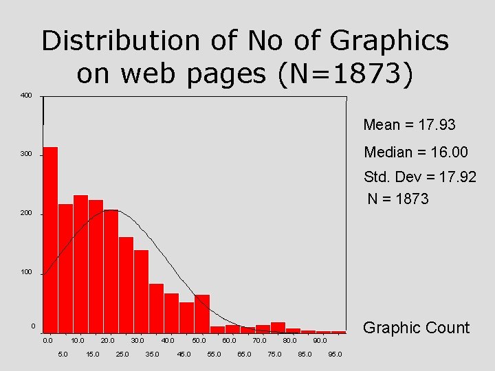
What can histograms tell you A convenient way to summarize data (especially for larger datasets) Shows the distribution of the variable in the population Gives an approximate idea of the summary and spread of the variable

Distribution of No of Graphics on web pages (N=1873) 400 Mean = 17. 93 Median = 16. 00 300 Std. Dev = 17. 92 N = 1873 200 100 Graphic Count 0 0. 0 10. 0 5. 0 20. 0 15. 0 30. 0 25. 0 40. 0 35. 0 50. 0 45. 0 60. 0 55. 0 70. 0 65. 0 80. 0 75. 0 90. 0 85. 0 95. 0

Statistics Review Mean and Median

Mean and Median Mean is arithmetic average, median is 50% point Mean is point where graph balances Mean shifts around, Median does not shift much, is more stable Computing Median: for odd numbered N find middle number For even numbered N interpolate between middle 2, e. g. if it is 7 and 9, then 8 is the median

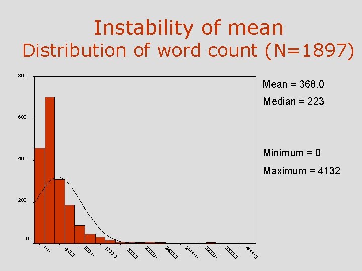
Instability of mean Distribution of word count (N=1897) 800 Mean = 368. 0 Median = 223 600 Minimum = 0 400 Maximum = 4132 200 0 WORDCNT 2. 0 00 40 . 0 00 36 . 0 00 32 . 0 00 28 . 0 00 24 . 0 00 20 . 0 00 16 . 0 00 12 0 0. 80 0 0. 40 0 0.

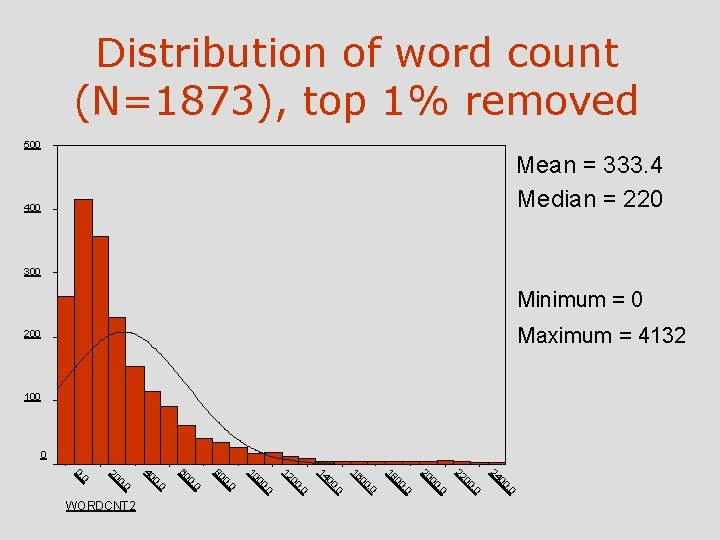
Distribution of word count (N=1873), top 1% removed 500 Mean = 333. 4 Median = 220 400 300 Minimum = 0 Maximum = 4132 200 100 0. 0 00 24 . 0 00 22 . 0 00 20 . 0 00 18 . 0 00 16 . 0 00 14 . 0 00 12 . 0 00 10 0 0. 80 0 0. 60 0 0. 40 0 0. 20 0 0. WORDCNT 2

Statistics Review Standard Deviation

Standard Deviation: a measure of spread The SD says how far away numbers on a list are from their average. Most entries on the list will be somewhere around one SD away from the average. Very few will be more than two or three SD’s away.

Properties of the standard deviation • The standard deviation is in the same units as the mean • The standard deviation is inversely related to sample size (therefore as a measure of spread it is biased) • In normally distributed data 68% of the sample lies within 1 SD

Statistics Review Normal Probability Curve

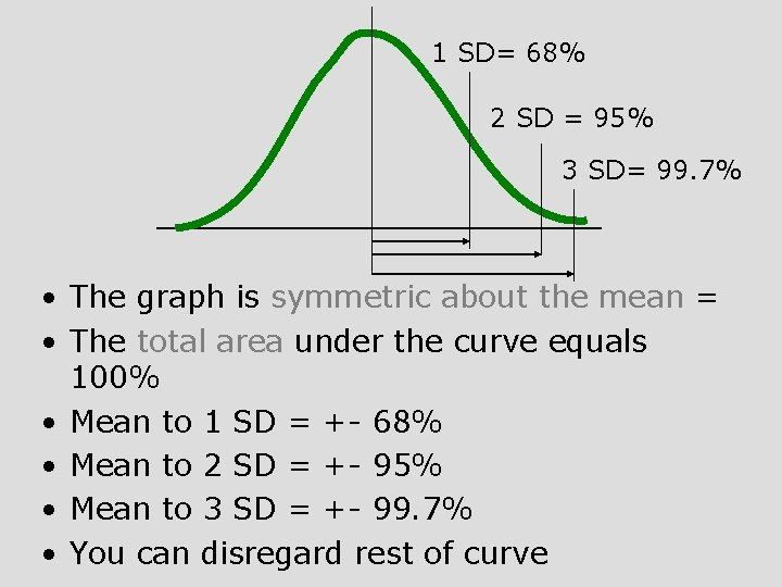
Properties of the Normal Probability Curve • The graph is symmetric about the mean (the part to the right is a mirror image of the part to the left) • The total area under the curve equals 100% • Curve is always above horizontal axis • Appears to stop after a certain point (the curve gets really low)

1 SD= 68% 2 SD = 95% 3 SD= 99. 7% • The graph is symmetric about the mean = • The total area under the curve equals 100% • Mean to 1 SD = +- 68% • Mean to 2 SD = +- 95% • Mean to 3 SD = +- 99. 7% • You can disregard rest of curve

It is a remarkable fact that many histograms in real life tend to follow the Normal Curve. For such histograms, the mean and SD are good summary statistics. The average pins down the center, while the SD gives the spread. For histogram which do not follow the normal Curve, the mean and SD are not good summary statistics. What when the histogram is not normal. . .

Use inter quartile range 75 th percentile - 25 th percentile Can be used when SD is too influenced by outliers Note. A percentile is a score below which a certain % of sample is

Statistics Review Population and Sample

An investigator usually wants to generalize about a class of individuals/things (the population) For example: in forecasting the results of elections, population is all eligible voters

• Usually there are some numerical facts about the population (parameters) which you want to estimate • You can do that by measuring the same aspect in the sample (statistic) • Depending on the accuracy of your measurement, and how representative your sample is, you can make inferences about the population

Statistics Review Scatter Plots and Correlations

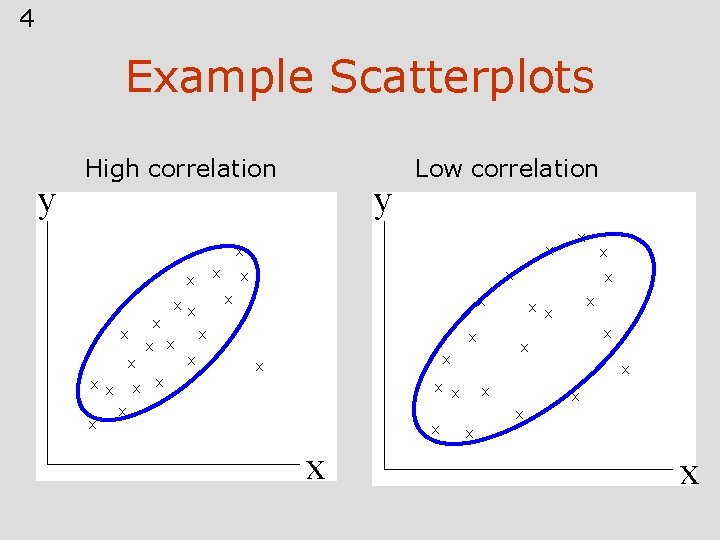
4 Example Scatterplots y High correlation y Low correlation x x x x x x x x x x x

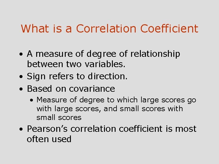
What is a Correlation Coefficient • A measure of degree of relationship between two variables. • Sign refers to direction. • Based on covariance • Measure of degree to which large scores go with large scores, and small scores with small scores • Pearson’s correlation coefficient is most often used

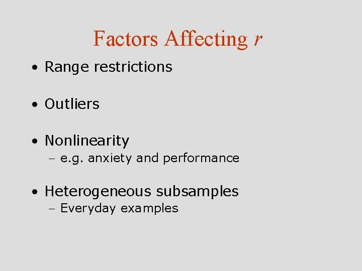
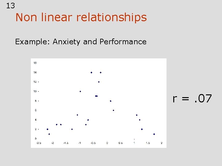
Factors Affecting r • Range restrictions • Outliers • Nonlinearity - e. g. anxiety and performance • Heterogeneous subsamples - Everyday examples

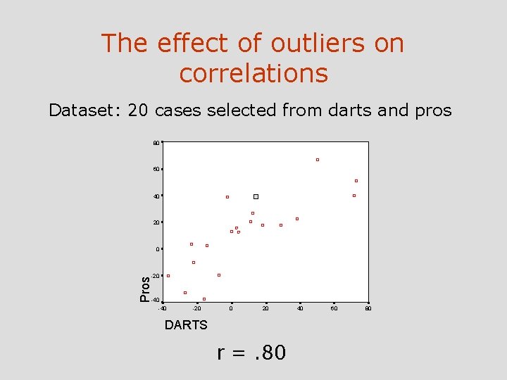
The effect of outliers on correlations Dataset: 20 cases selected from darts and pros 80 60 40 20 0 Pros -20 -40 -20 0 20 DARTS r =. 80 40 60 80

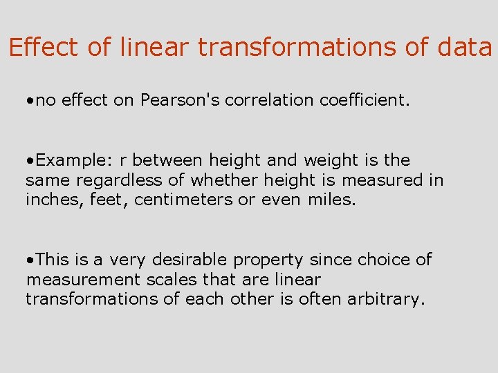
Effect of linear transformations of data • no effect on Pearson's correlation coefficient. • Example: r between height and weight is the same regardless of whether height is measured in inches, feet, centimeters or even miles. • This is a very desirable property since choice of measurement scales that are linear transformations of each other is often arbitrary.

13 Non linear relationships Example: Anxiety and Performance r =. 07

The interpretation of a correlation coefficient • Ranges from – 1 to 1 • No correlation in the data means you will get a is 0 r or near it • Suffers from sampling error (like everything else!). So you need to estimate true population correlation from the sample correlation.

Statistics Review Hypothesis Testing

Null and Alternative Hypothesis • Sampling error implies that sometimes the results we obtain will be due to chance (since not every sample will accurately resemble the population) • The null hypothesis expresses the idea that an observed difference is due to chance. • For example: There is no difference between the norms regarding the use of email and voice mail

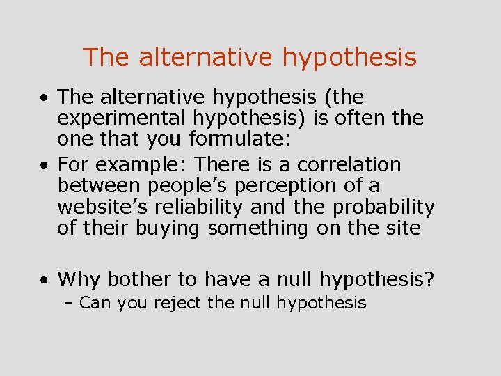
The alternative hypothesis • The alternative hypothesis (the experimental hypothesis) is often the one that you formulate: • For example: There is a correlation between people’s perception of a website’s reliability and the probability of their buying something on the site • Why bother to have a null hypothesis? – Can you reject the null hypothesis

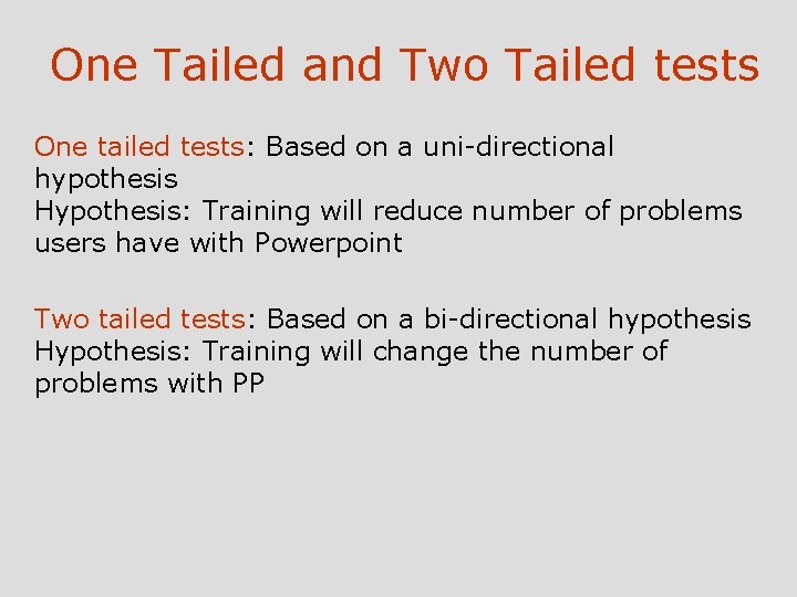
One Tailed and Two Tailed tests One tailed tests: Based on a uni-directional hypothesis Hypothesis: Training will reduce number of problems users have with Powerpoint Two tailed tests: Based on a bi-directional hypothesis Hypothesis: Training will change the number of problems with PP

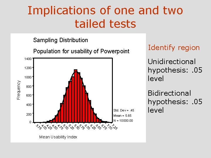
Implications of one and two tailed tests Sampling Distribution Population for usability of Powerpoint 1400 Unidirectional hypothesis: . 05 level 1200 1000 Frequency Identify region 800 600 400 Std. Dev =. 45 200 Mean = 5. 65 N = 10000. 00 0 25 7. 00 7. 75 6. 50 6. 25 6. 00 6. 75 5. 50 5. 25 5. 00 5. 75 4. 50 4. 25 4. 00 4. 75 3. Mean Usability Index Bidirectional hypothesis: . 05 level

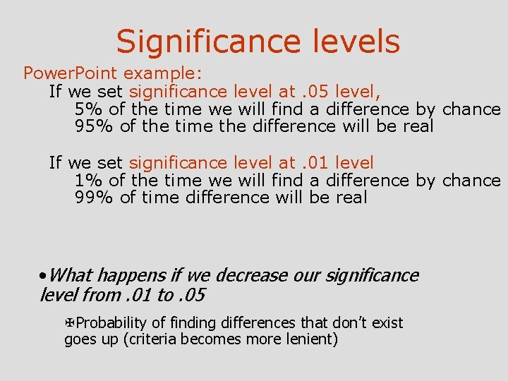
Significance levels Power. Point example: If we set significance level at. 05 level, 5% of the time we will find a difference by chance 95% of the time the difference will be real If we set significance level at. 01 level 1% of the time we will find a difference by chance 99% of time difference will be real • What happens if we decrease our significance level from. 01 to. 05 XProbability of finding differences that don’t exist goes up (criteria becomes more lenient)

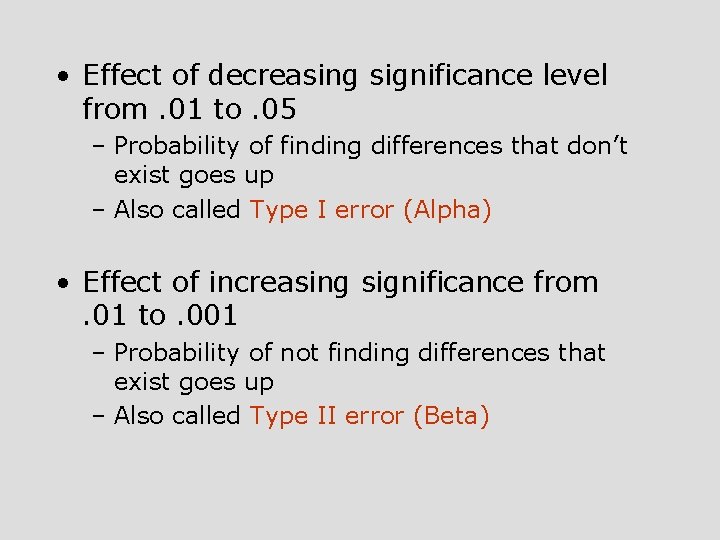
• Effect of decreasing significance level from. 01 to. 05 – Probability of finding differences that don’t exist goes up – Also called Type I error (Alpha) • Effect of increasing significance from. 01 to. 001 – Probability of not finding differences that exist goes up – Also called Type II error (Beta)

Significance levels for usability • For usability, if you are set out to find problems: setting lenient criteria might work better (you will identify more problems)

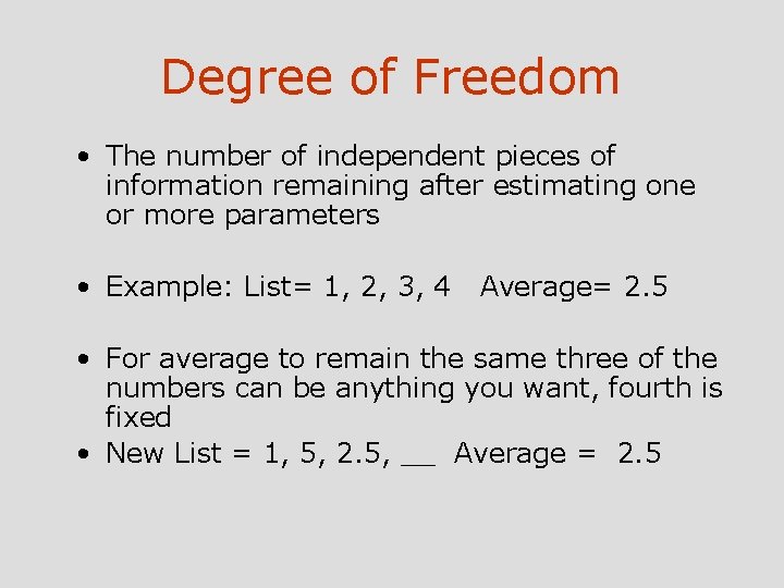
Degree of Freedom • The number of independent pieces of information remaining after estimating one or more parameters • Example: List= 1, 2, 3, 4 Average= 2. 5 • For average to remain the same three of the numbers can be anything you want, fourth is fixed • New List = 1, 5, 2. 5, __ Average = 2. 5

Statistics Review Comparing Means: t tests

Major Points • T tests: are differences significant? • One sample t tests, comparing one mean to population • Within subjects test: Comparing mean in condition 1 to mean in condition 2 • Between Subjects test: Comparing mean in condition 1 to mean in condition 2

One sample t test • Mean of population known, but standard deviation (SD) not known • Compute t statistic • Compare t to tabled values (for relevant degree of freedom) which show critical values of t

Factors Affecting t • Difference between sample and population means • Magnitude of sample variance • Sample size

Factors Affecting Decision • Significance level • One-tailed versus two-tailed test

Within subjects/ Repeated Measures / Related Samples t test • Correlation between before and after scores – Causes a change in the statistic we can use Advantages of within subject designs • Eliminate subject-to-subject variability • Control for extraneous variables • Need fewer subjects

Disadvantages of Within Subjects • • Order effects Carry-over effects Subjects no longer naïve Change may just be a function of time • Sometimes not logically possible

Between subjects t test • Distribution of differences between means • Heterogeneity of Variance • Nonnormality

Assumptions of Between Subjects t tests • Two major assumptions – Both groups are sampled from populations with the same variance • “homogeneity of variance” – Both groups are sampled from normal populations • Assumption of normality – Frequently violated with little harm.

Statistics Review Analysis of Variance

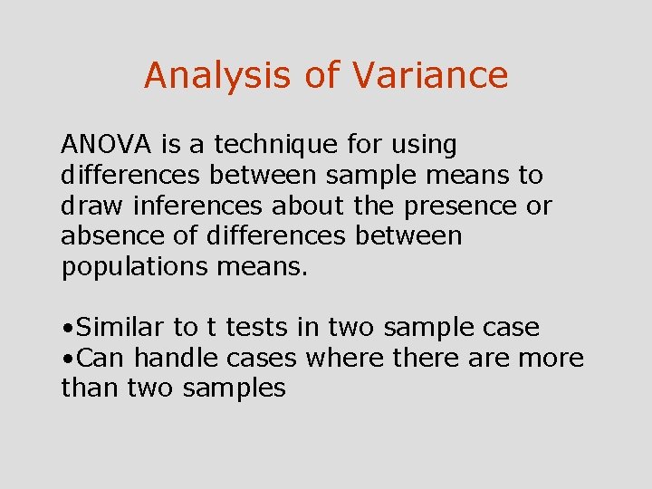
Analysis of Variance ANOVA is a technique for using differences between sample means to draw inferences about the presence or absence of differences between populations means. • Similar to t tests in two sample case • Can handle cases where there are more than two samples

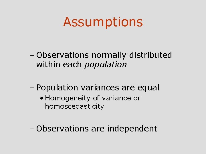
Assumptions – Observations normally distributed within each population – Population variances are equal • Homogeneity of variance or homoscedasticity – Observations are independent

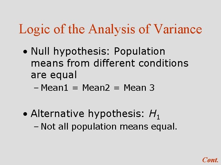
Logic of the Analysis of Variance • Null hypothesis: Population means from different conditions are equal – Mean 1 = Mean 2 = Mean 3 • Alternative hypothesis: H 1 – Not all population means equal. Cont.

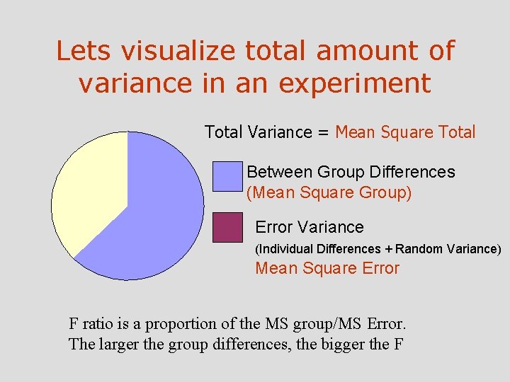
Lets visualize total amount of variance in an experiment Total Variance = Mean Square Total Between Group Differences (Mean Square Group) Error Variance (Individual Differences + Random Variance) Mean Square Error F ratio is a proportion of the MS group/MS Error. The larger the group differences, the bigger the F

When there are more than two groups • Significant F only shows that not all groups are equal – We want to know what groups are different. • Such procedures are designed to control familywise error rate. – Familywise error rate defined – Contrast with per comparison error rate

Multiple Comparisons • The more tests we run the more likely we are to make Type I error. – Good reason to hold down number of tests

How to make inferences • What are significant effects in your results? • If one t test is significant, check the distribution, where does the difference lie: Is it in the mean, is it the SD, does one variable have much greater range than another. • Next conduct another independent analysis which can verify finding. For example: Check the