Statistics Principles of Engineering 2012 Project Lead The

Statistics Principles of Engineering © 2012 Project Lead The Way, Inc.

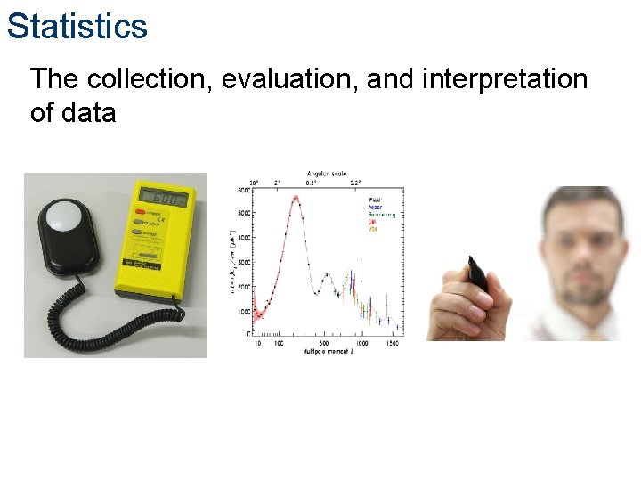
Statistics The collection, evaluation, and interpretation of data

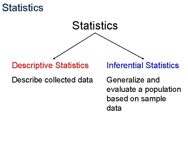
Statistics Descriptive Statistics Inferential Statistics Describe collected data Generalize and evaluate a population based on sample data

Data Categorical or Qualitative Data Values that possess names or labels Color of M&M’s, breed of dog, etc. Numerical or Quantitative Data Values that represent a measurable quantity Population, number of M&M’s, number of defective parts, etc.

Data Collection Sampling • Random • Systematic • Stratified • Cluster • Convenience

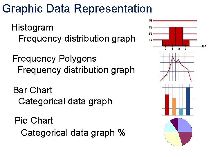
Graphic Data Representation Histogram Frequency distribution graph Frequency Polygons Frequency distribution graph Bar Chart Categorical data graph Pie Chart Categorical data graph %

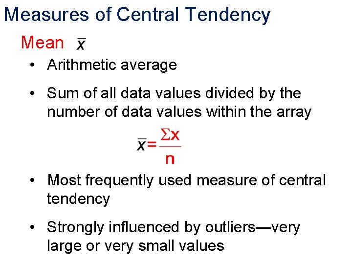
Measures of Central Tendency Mean • Arithmetic average • Sum of all data values divided by the number of data values within the array • Most frequently used measure of central tendency • Strongly influenced by outliers—very large or very small values

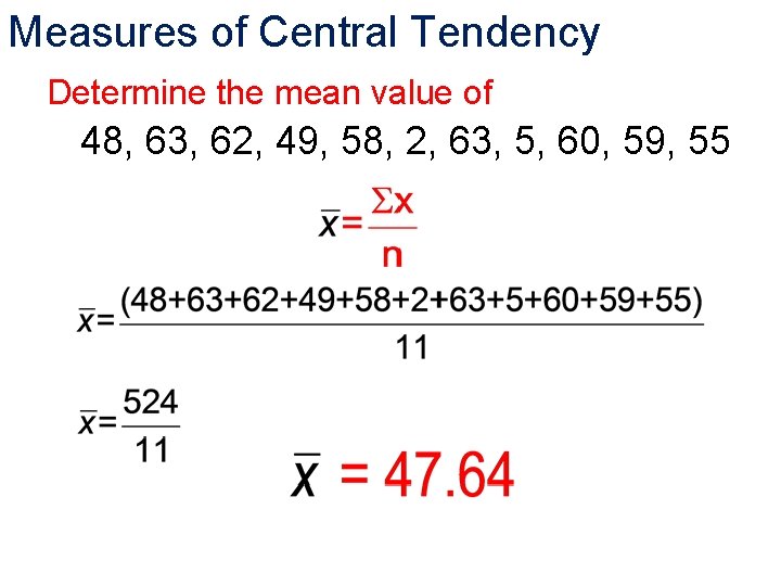
Measures of Central Tendency Determine the mean value of 48, 63, 62, 49, 58, 2, 63, 5, 60, 59, 55

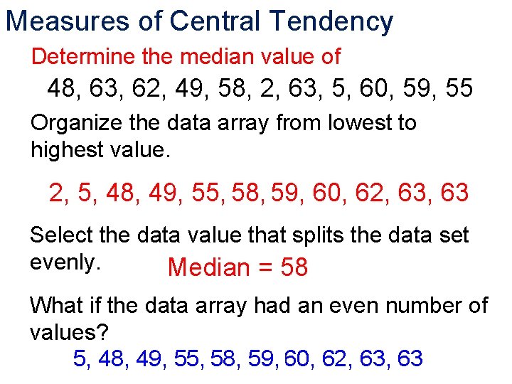
Measures of Central Tendency Median • Data value that divides a data array into two equal groups • Data values must be ordered from lowest to highest • Useful in situations with skewed data and outliers (e. g. , wealth management)

Measures of Central Tendency Determine the median value of 48, 63, 62, 49, 58, 2, 63, 5, 60, 59, 55 Organize the data array from lowest to highest value. 2, 5, 48, 49, 55, 58, 59, 60, 62, 63 Select the data value that splits the data set evenly. Median = 58 What if the data array had an even number of values? 5, 48, 49, 55, 58, 59, 60, 62, 63

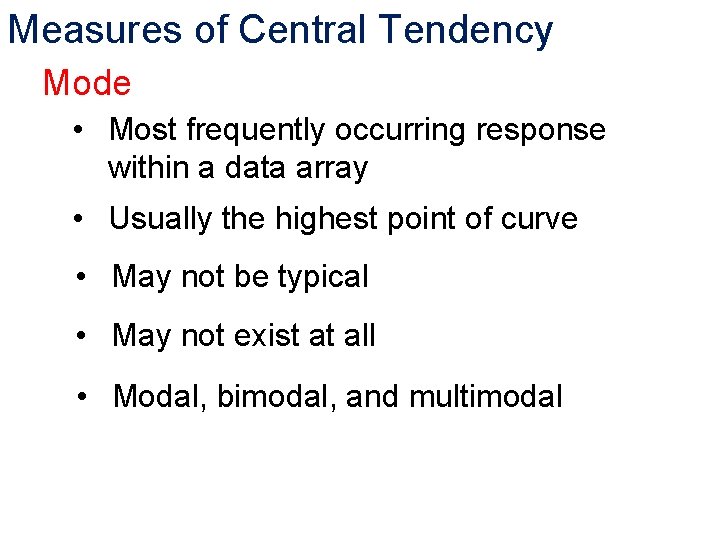
Measures of Central Tendency Mode • Most frequently occurring response within a data array • Usually the highest point of curve • May not be typical • May not exist at all • Modal, bimodal, and multimodal

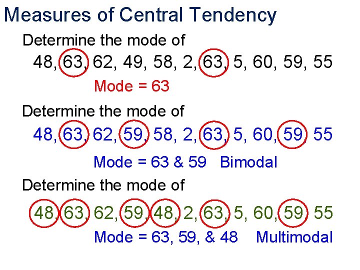
Measures of Central Tendency Determine the mode of 48, 63, 62, 49, 58, 2, 63, 5, 60, 59, 55 Mode = 63 Determine the mode of 48, 63, 62, 59, 58, 2, 63, 5, 60, 59, 55 Mode = 63 & 59 Bimodal Determine the mode of 48, 63, 62, 59, 48, 2, 63, 5, 60, 59, 55 Mode = 63, 59, & 48 Multimodal

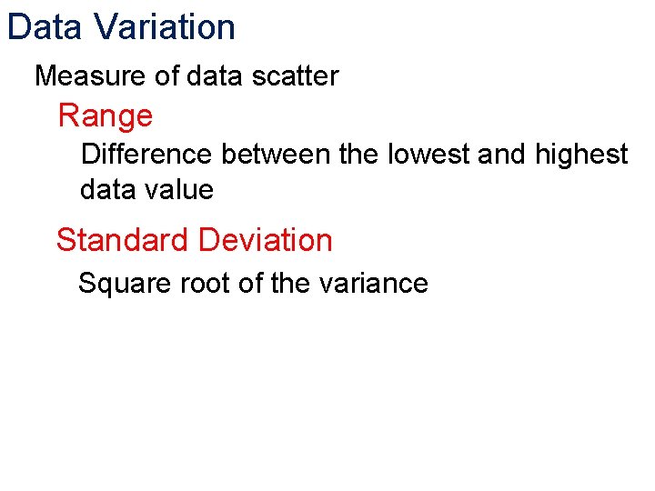
Data Variation Measure of data scatter Range Difference between the lowest and highest data value Standard Deviation Square root of the variance

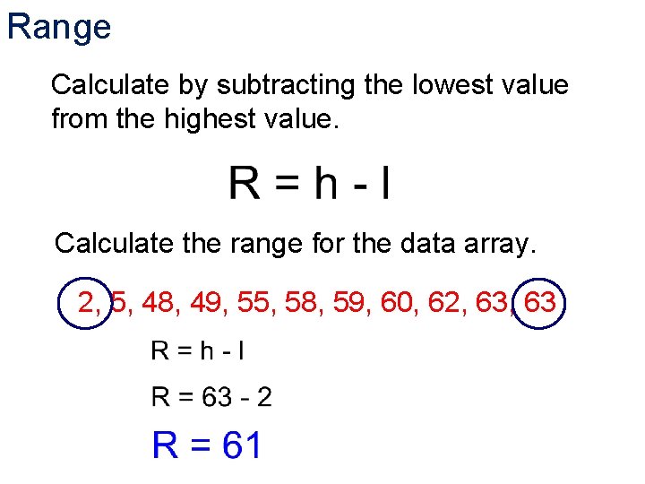
Range Calculate by subtracting the lowest value from the highest value. Calculate the range for the data array. 2, 5, 48, 49, 55, 58, 59, 60, 62, 63

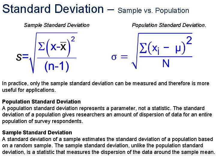
Standard Deviation – Sample vs. Population Sample Standard Deviation Population Standard Deviation. In practice, only the sample standard deviation can be measured and therefore is more useful for applications. Population Standard Deviation A population standard deviation represents a parameter, not a statistic. The standard deviation of a population gives researchers an amount of dispersion of data for an entire population of survey respondents. Sample Standard Deviation A standard deviation of a sample estimates the standard deviation of a population based on a random sample. The sample standard deviation, unlike the population standard deviation, is a statistic that measures the dispersion of the data around the sample mean.

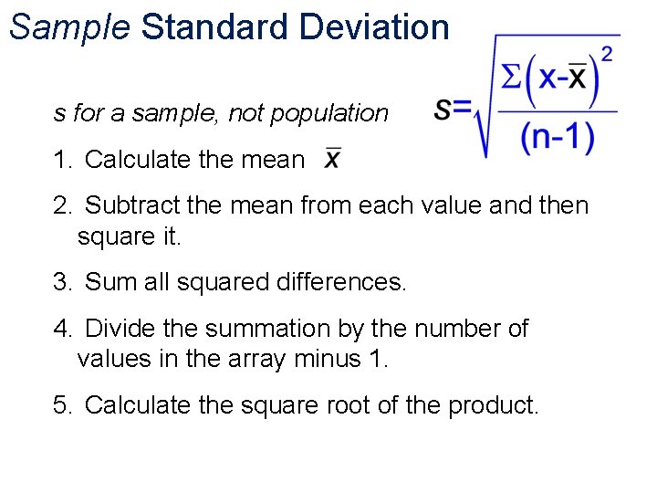
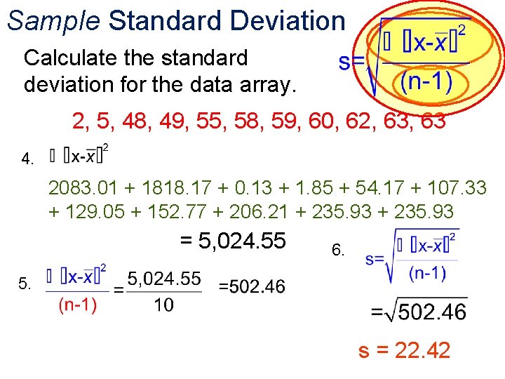
Sample Standard Deviation s for a sample, not population 1. Calculate the mean 2. Subtract the mean from each value and then square it. 3. Sum all squared differences. 4. Divide the summation by the number of values in the array minus 1. 5. Calculate the square root of the product.

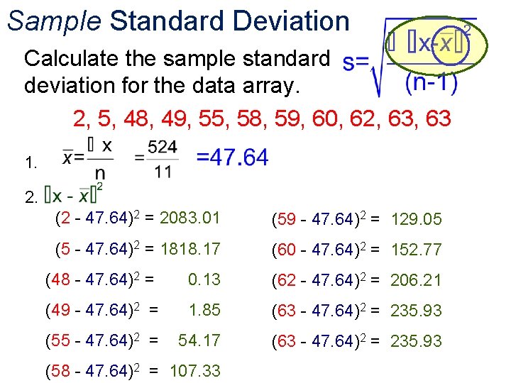
Sample Standard Deviation Calculate the sample standard deviation for the data array. 2, 5, 48, 49, 55, 58, 59, 60, 62, 63 1. 2. (2 - 47. 64)2 = 2083. 01 (59 - 47. 64)2 = 129. 05 (5 - 47. 64)2 = 1818. 17 (60 - 47. 64)2 = 152. 77 (48 - 47. 64)2 = 0. 13 (62 - 47. 64)2 = 206. 21 (49 - 47. 64)2 = 1. 85 (63 - 47. 64)2 = 235. 93 (55 - 47. 64)2 = 54. 17 (63 - 47. 64)2 = 235. 93 (58 - 47. 64)2 = 107. 33

Sample Standard Deviation Calculate the standard deviation for the data array. 2, 5, 48, 49, 55, 58, 59, 60, 62, 63 4. 2083. 01 + 1818. 17 + 0. 13 + 1. 85 + 54. 17 + 107. 33 + 129. 05 + 152. 77 + 206. 21 + 235. 93 = 5, 024. 55 6. 5. s = 22. 42

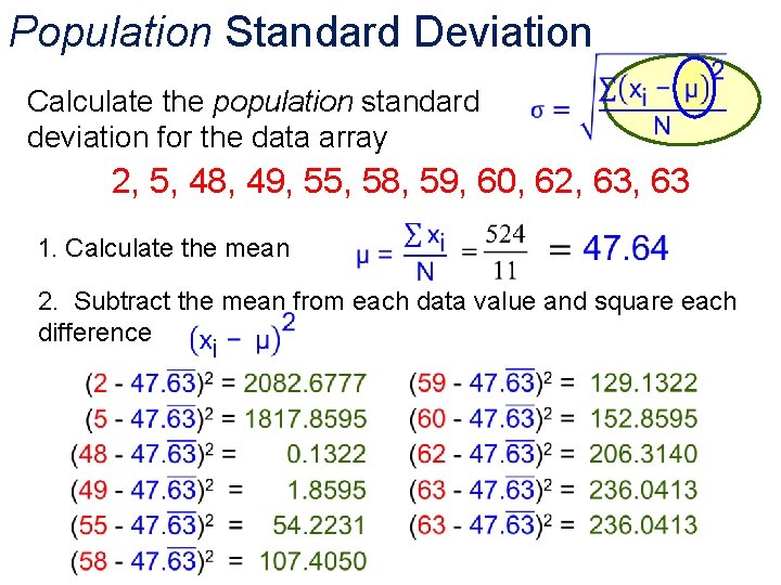
Population Standard Deviation Calculate the population standard deviation for the data array 2, 5, 48, 49, 55, 58, 59, 60, 62, 63 1. Calculate the mean 2. Subtract the mean from each data value and square each difference

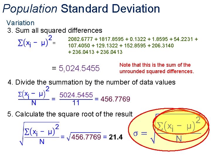
Population Standard Deviation Variation 3. Sum all squared differences 2082. 6777 + 1817. 8595 + 0. 1322 + 1. 8595 + 54. 2231 + 107. 4050 + 129. 1322 + 152. 8595 + 206. 3140 + 236. 0413 = 5, 024. 5455 Note that this is the sum of the unrounded squared differences. 4. Divide the summation by the number of data values 5. Calculate the square root of the result

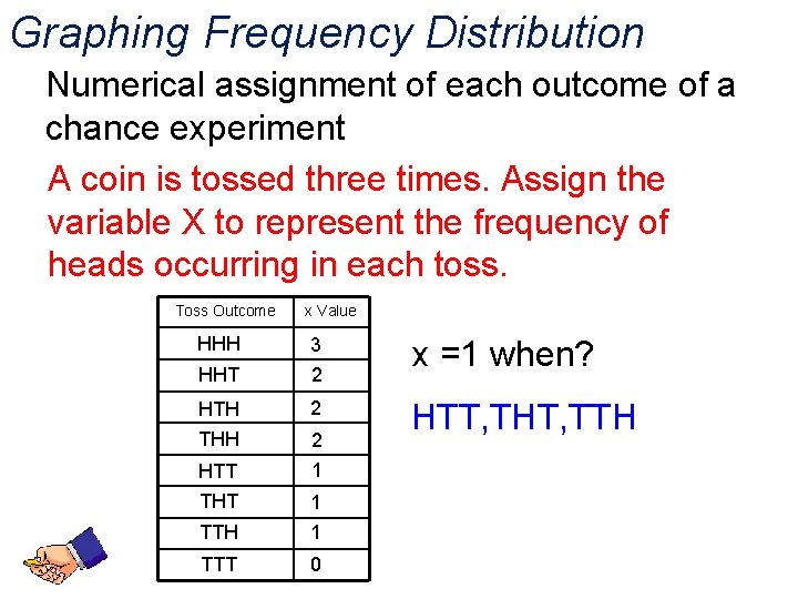
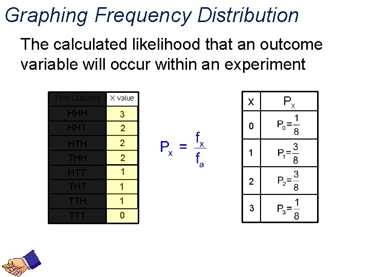
Graphing Frequency Distribution Numerical assignment of each outcome of a chance experiment A coin is tossed three times. Assign the variable X to represent the frequency of heads occurring in each toss. Toss Outcome HHH HHT HTH THH x Value 3 2 x =1 when? 2 HTT, THT, TTH 2 1 HTT THT 1 TTH 1 TTT 0

Graphing Frequency Distribution The calculated likelihood that an outcome variable will occur within an experiment Toss Outcome X value HHH 3 2 HHT HTH THH 2 2 1 HTT THT 1 TTH 1 TTT 0 x 0 1 2 3 Px

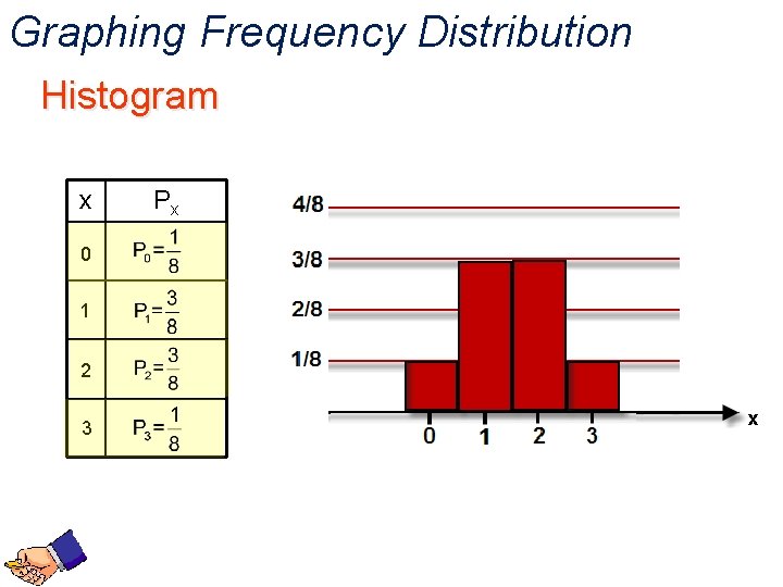
Graphing Frequency Distribution Histogram x Px 0 1 2 3 x

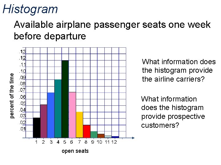
Histogram Available airplane passenger seats one week before departure percent of the time What information does the histogram provide the airline carriers? What information does the histogram provide prospective customers? open seats