Statistics Part II John Van Meter Ph D

Statistics Part II John Van. Meter, Ph. D. Center for Functional and Molecular Imaging Georgetown University Medical Center

Multiple Comparisons Problem • The p-value gives the likelihood that the changes in the MRI signal are related to the task • If the p = 0. 05 there is a 5% chance that we wrongly classify a voxel as active • If we look at 100 voxels then at least 5 of them will be significant by chance alone

Multiple Comparisons Problem • A voxel-by-voxel based analysis requires over 100, 000 t-tests to be performed • A correction must be applied otherwise we will have ~5, 000 random voxels that are unrelated to the task that will appear to be activated • Can reduce number of t-tests if we know where to test - such as just inside the brain or specific regions

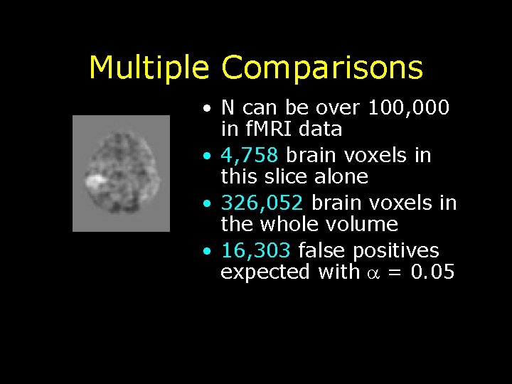
Multiple Comparisons • N can be over 100, 000 in f. MRI data • 4, 758 brain voxels in this slice alone • 326, 052 brain voxels in the whole volume • 16, 303 false positives expected with = 0. 05

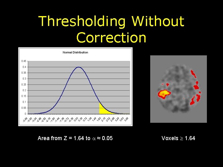
Thresholding Without Correction Area from Z = 1. 64 to ≈ 0. 05 Voxels 1. 64

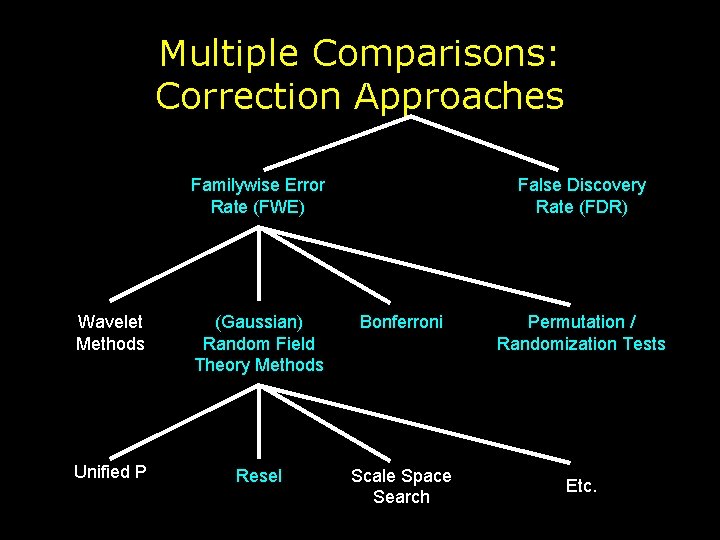
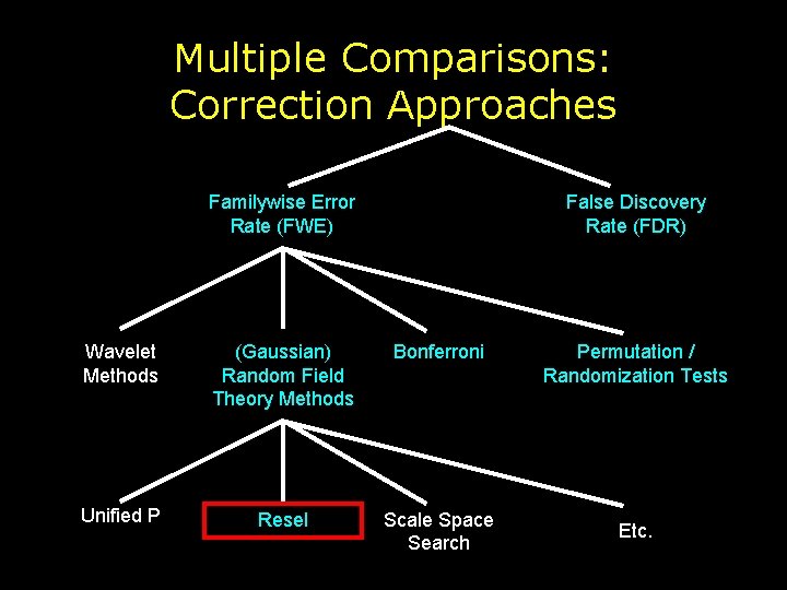
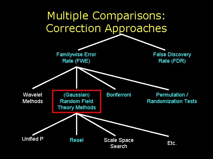
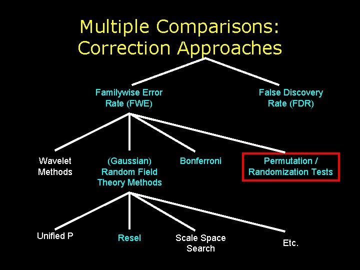
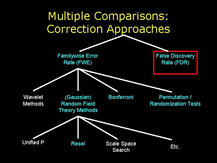
Multiple Comparisons: Correction Approaches Familywise Error Rate (FWE) False Discovery Rate (FDR) Wavelet Methods (Gaussian) Random Field Theory Methods Bonferroni Unified P Resel Scale Space Search Permutation / Randomization Tests Etc.

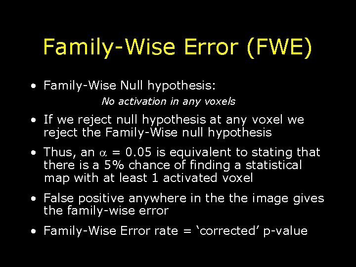
Family-Wise Error (FWE) • Family-Wise Null hypothesis: No activation in any voxels • If we reject null hypothesis at any voxel we reject the Family-Wise null hypothesis • Thus, an = 0. 05 is equivalent to stating that there is a 5% chance of finding a statistical map with at least 1 activated voxel • False positive anywhere in the image gives the family-wise error • Family-Wise Error rate = ‘corrected’ p-value

Multiple Comparisons: Correction Approaches Familywise Error Rate (FWE) False Discovery Rate (FDR) Wavelet Methods (Gaussian) Random Field Theory Methods Bonferroni Unified P Resel Scale Space Search Permutation / Randomization Tests Etc.

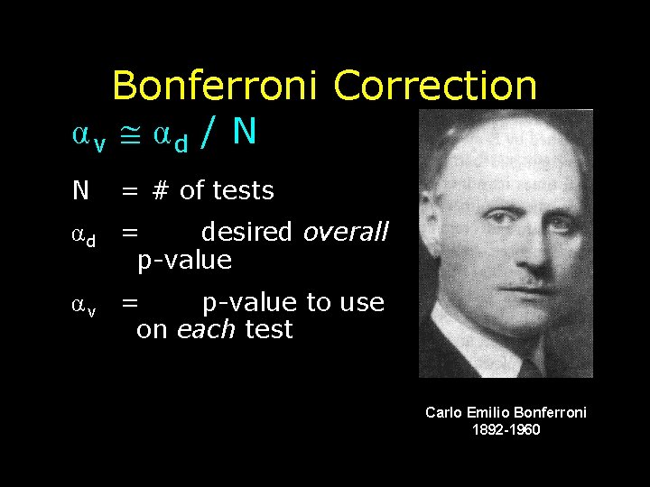
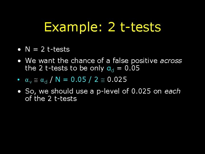
Bonferroni Correction αv αd / N N = # of tests αd = desired overall p-value αv = p-value to use on each test Carlo Emilio Bonferroni 1892 -1960

Example: 2 t-tests • N = 2 t-tests • We want the chance of a false positive across the 2 t-tests to be only αd = 0. 05 • α v α d / N = 0. 05 / 2 0. 025 • So, we should use a p-level of 0. 025 on each of the 2 t-tests

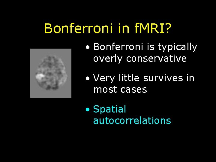
Bonferroni in f. MRI? • Bonferroni is typically overly conservative • Very little survives in most cases • Spatial autocorrelations

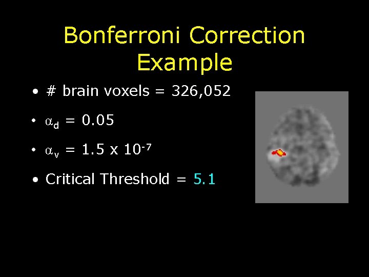
Bonferroni Correction Example • # brain voxels = 326, 052 • α d = 0. 05 • α v = 1. 5 x 10 -7 • Critical Threshold = 5. 1

Multiple Comparisons: Correction Approaches Familywise Error Rate (FWE) False Discovery Rate (FDR) Wavelet Methods (Gaussian) Random Field Theory Methods Bonferroni Unified P Resel Scale Space Search Permutation / Randomization Tests Etc.

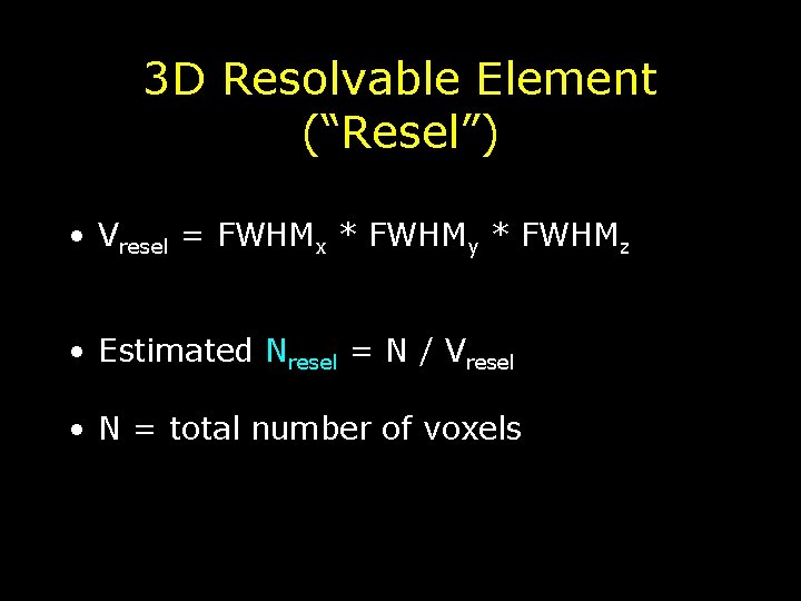
3 D Resolvable Element (“Resel”) • Vresel = FWHMx * FWHMy * FWHMz • Estimated Nresel = N / Vresel • N = total number of voxels

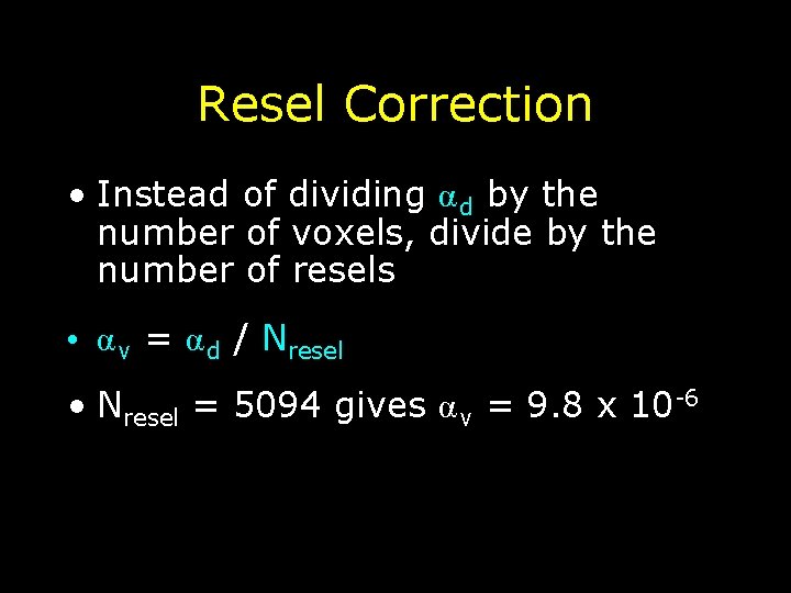
Resel Correction • Instead of dividing α d by the number of voxels, divide by the number of resels • α v = α d / Nresel • Nresel = 5094 gives α v = 9. 8 x 10 -6

Multiple Comparisons: Correction Approaches Familywise Error Rate (FWE) False Discovery Rate (FDR) Wavelet Methods (Gaussian) Random Field Theory Methods Bonferroni Unified P Resel Scale Space Search Permutation / Randomization Tests Etc.

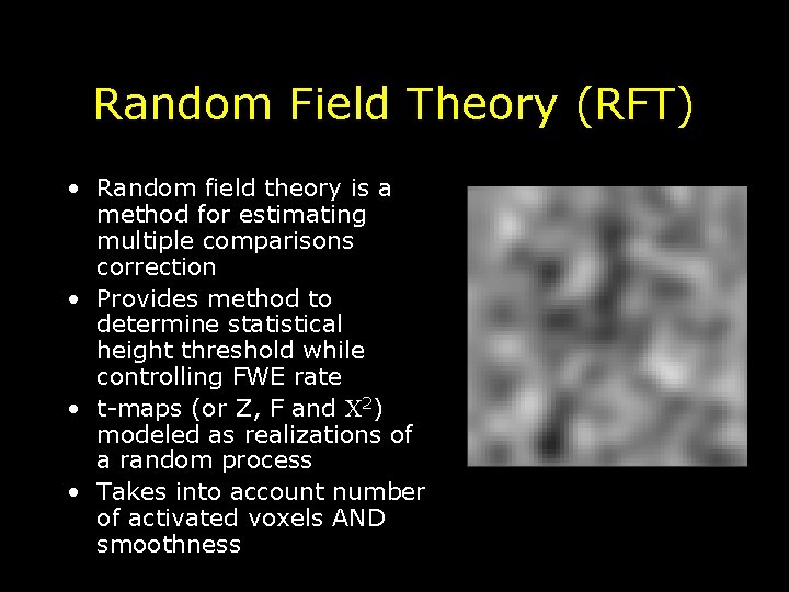
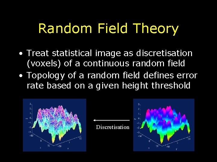
Random Field Theory (RFT) • Random field theory is a method for estimating multiple comparisons correction • Provides method to determine statistical height threshold while controlling FWE rate • t-maps (or Z, F and 2) modeled as realizations of a random process • Takes into account number of activated voxels AND smoothness

Random Field Theory • Treat statistical image as discretisation (voxels) of a continuous random field • Topology of a random field defines error rate based on a given height threshold Discretisation

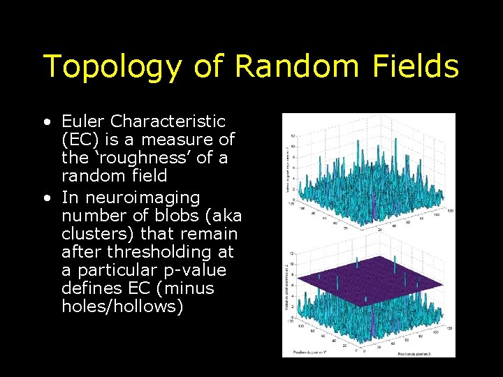
Topology of Random Fields • Euler Characteristic (EC) is a measure of the ‘roughness’ of a random field • In neuroimaging number of blobs (aka clusters) that remain after thresholding at a particular p-value defines EC (minus holes/hollows)

Euler Characteristic (EC) Topological measure – threshold an image at u - EC = # blobs - holes/hollows

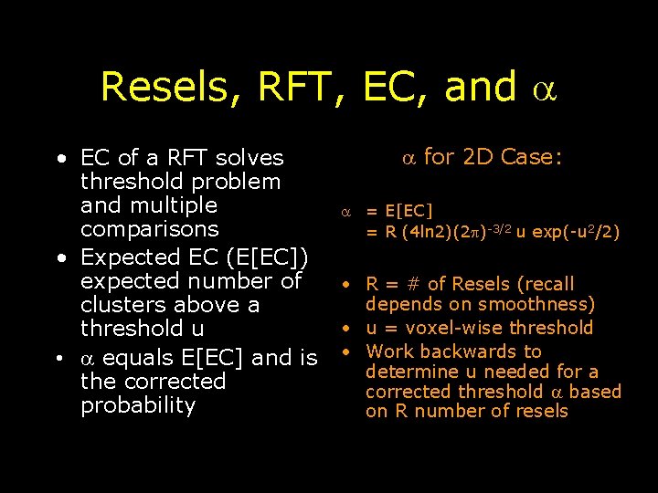
Resels, RFT, EC, and • EC of a RFT solves threshold problem and multiple comparisons • Expected EC (E[EC]) expected number of clusters above a threshold u • equals E[EC] and is the corrected probability for 2 D Case: = E[EC] = R (4 ln 2)(2 )-3/2 u exp(-u 2/2) • R = # of Resels (recall depends on smoothness) • u = voxel-wise threshold • Work backwards to determine u needed for a corrected threshold based on R number of resels

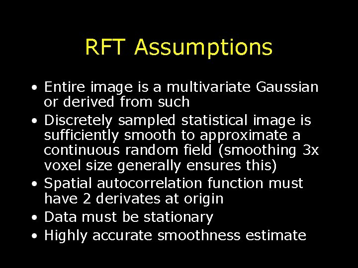
RFT Assumptions • Entire image is a multivariate Gaussian or derived from such • Discretely sampled statistical image is sufficiently smooth to approximate a continuous random field (smoothing 3 x voxel size generally ensures this) • Spatial autocorrelation function must have 2 derivates at origin • Data must be stationary • Highly accurate smoothness estimate

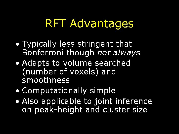
RFT Advantages • Typically less stringent that Bonferroni though not always • Adapts to volume searched (number of voxels) and smoothness • Computationally simple • Also applicable to joint inference on peak-height and cluster size

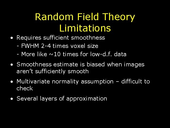
Random Field Theory Limitations • Requires sufficient smoothness - FWHM 2 -4 times voxel size - More like ~10 times for low-d. f. data • Smoothness estimate is biased when images aren’t sufficiently smooth • Multivariate normality assumption – difficult to check • Several layers of approximation

Multiple Comparisons: Correction Approaches Familywise Error Rate (FWE) False Discovery Rate (FDR) Wavelet Methods (Gaussian) Random Field Theory Methods Bonferroni Unified P Resel Scale Space Search Permutation / Randomization Tests Etc.

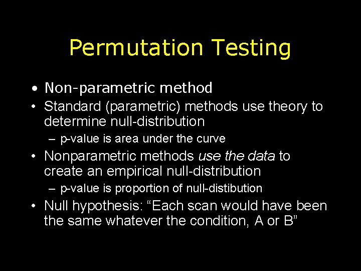
Permutation Testing • Non-parametric method • Standard (parametric) methods use theory to determine null-distribution – p-value is area under the curve • Nonparametric methods use the data to create an empirical null-distribution – p-value is proportion of null-distibution • Null hypothesis: “Each scan would have been the same whatever the condition, A or B”

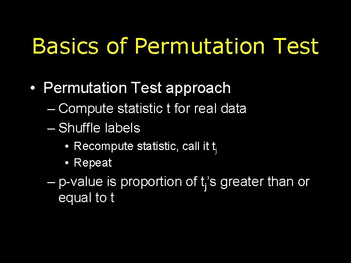
Basics of Permutation Test • Permutation Test approach – Compute statistic t for real data – Shuffle labels • Recompute statistic, call it tj • Repeat – p-value is proportion of tj’s greater than or equal to t

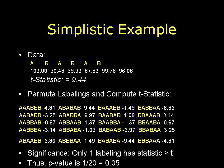
Simplistic Example • Data: A B A B 103. 00 90. 48 99. 93 87. 83 99. 76 96. 06 t-Statistic: = 9. 44 • Permute Labelings and Compute t-Statistic: AAABBB 4. 81 AABABB -3. 25 AABBAB -0. 67 AABBBA -3. 14 ABABAB 9. 44 ABABBA 6. 97 ABBAAB 1. 37 ABBABA -1. 09 BAAABB -1. 49 BAABAB 1. 09 BAABBA -1. 37 BABAAB -6. 97 BABBAA -6. 86 BBAAAB 3. 14 BBAABA 0. 67 BBABAA 3. 25 ABAABB 6. 86 ABBBAA 1. 49 BABABA -9. 44 BBBAAA -4. 81 • Significance: Only 1 labeling has statistic ≥ t • Thus, p-value is 1/20 = 0. 05

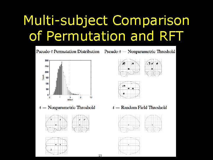
Multi-subject Comparison of Permutation and RFT

Permutation Test Assumptions and Disadvantages • Only assumption required is exchangeability under Ho • Not valid for single subject f. MRI as data is temporally autocorrelated • Valid for multi-subject f. MRI analyses (random effects) • Main disadvantage computationally intensive! • Implemented in Sn. PM toolbox

Multiple Comparisons: Correction Approaches Familywise Error Rate (FWE) False Discovery Rate (FDR) Wavelet Methods (Gaussian) Random Field Theory Methods Bonferroni Unified P Resel Scale Space Search Permutation / Randomization Tests Etc.

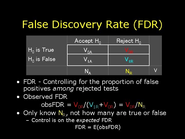
False Discovery Rate (FDR) H 0 is True H 0 is False Accept H 0 V 0 A V 1 A Reject H 0 V 0 R V 1 R NA NR V • FDR - Controlling for the proportion of false positives among rejected tests • Observed FDR obs. FDR = V 0 R/(V 1 R+V 0 R) = V 0 R/NR • Only know NR, not how many are true or false – Control is on the expected FDR = E(obs. FDR)

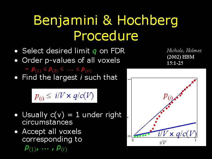
Benjamini & Hochberg Procedure • Select desired limit q on FDR • Order p-values of all voxels Nichols, Holmes (2002) HBM 15: 1 -25 • Find the largest i such that 1 – p(1) p(2) . . . p(V) p(i) i/V q/c(V) p-value i/V q/c(V) 0 • Usually c(v) = 1 under right circumstances • Accept all voxels corresponding to p(1), . . . , p(r) p(i) 0 i/V 1

Controlling FDR: Varying Signal Extent p= Signal Intensity 3. 0 z= Signal Extent 1. 0 Noise Smoothness 3. 0 1

Controlling FDR: Varying Signal Extent p= Signal Intensity 3. 0 z= Signal Extent 2. 0 Noise Smoothness 3. 0 2

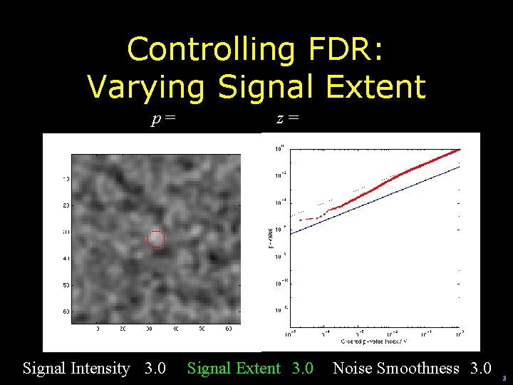
Controlling FDR: Varying Signal Extent p= Signal Intensity 3. 0 z= Signal Extent 3. 0 Noise Smoothness 3. 0 3

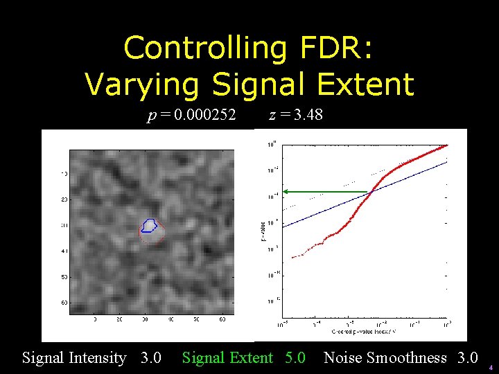
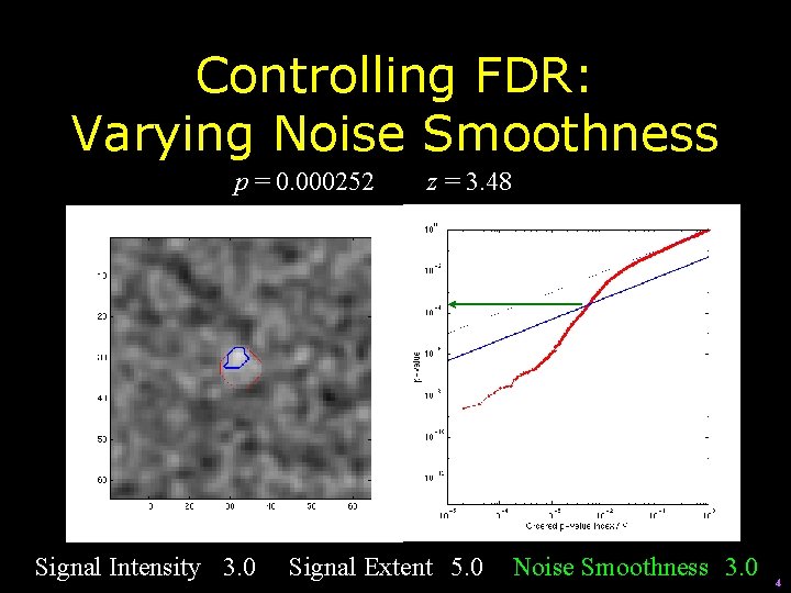
Controlling FDR: Varying Signal Extent p = 0. 000252 Signal Intensity 3. 0 z = 3. 48 Signal Extent 5. 0 Noise Smoothness 3. 0 4

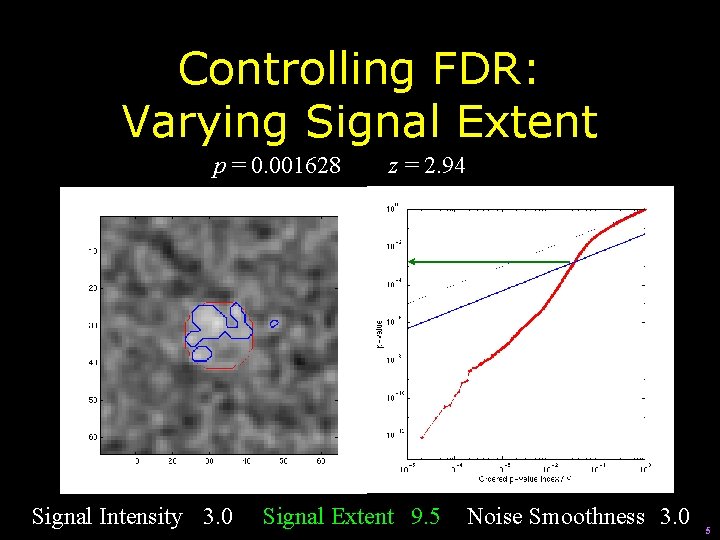
Controlling FDR: Varying Signal Extent p = 0. 001628 Signal Intensity 3. 0 z = 2. 94 Signal Extent 9. 5 Noise Smoothness 3. 0 5

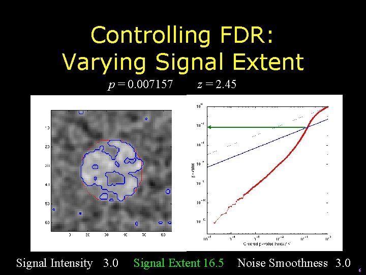
Controlling FDR: Varying Signal Extent p = 0. 007157 Signal Intensity 3. 0 z = 2. 45 Signal Extent 16. 5 Noise Smoothness 3. 0 6

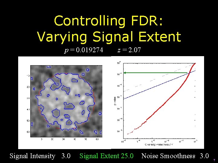
Controlling FDR: Varying Signal Extent p = 0. 019274 Signal Intensity 3. 0 z = 2. 07 Signal Extent 25. 0 Noise Smoothness 3. 0 7

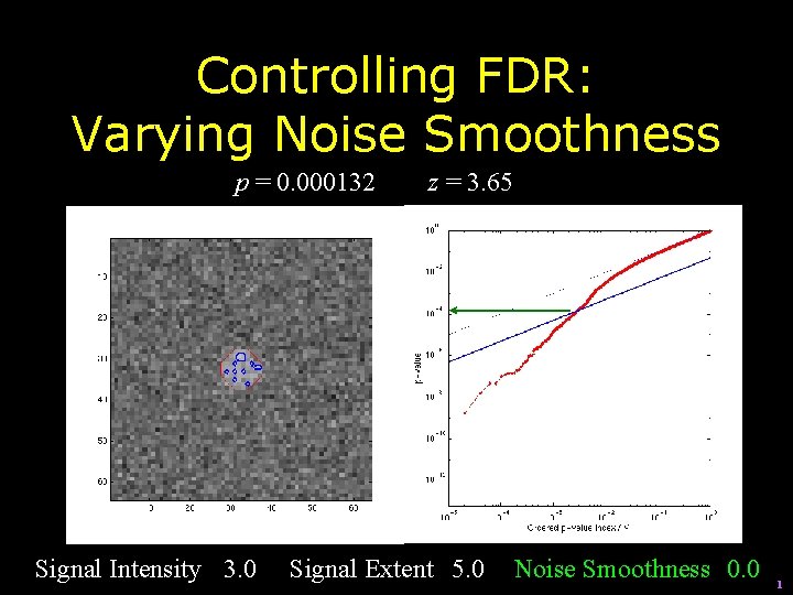
Controlling FDR: Varying Noise Smoothness p = 0. 000132 Signal Intensity 3. 0 z = 3. 65 Signal Extent 5. 0 Noise Smoothness 0. 0 1

Controlling FDR: Varying Noise Smoothness p = 0. 000169 Signal Intensity 3. 0 z = 3. 58 Signal Extent 5. 0 Noise Smoothness 1. 5 2

Controlling FDR: Varying Noise Smoothness p = 0. 000167 Signal Intensity 3. 0 z = 3. 59 Signal Extent 5. 0 Noise Smoothness 2. 0 3

Controlling FDR: Varying Noise Smoothness p = 0. 000252 Signal Intensity 3. 0 z = 3. 48 Signal Extent 5. 0 Noise Smoothness 3. 0 4

Controlling FDR: Varying Noise Smoothness p = 0. 000253 Signal Intensity 3. 0 z = 3. 48 Signal Extent 5. 0 Noise Smoothness 4. 0 5

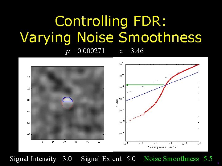
Controlling FDR: Varying Noise Smoothness p = 0. 000271 Signal Intensity 3. 0 z = 3. 46 Signal Extent 5. 0 Noise Smoothness 5. 5 6

Controlling FDR: Varying Noise Smoothness p = 0. 000274 Signal Intensity 3. 0 z = 3. 46 Signal Extent 5. 0 Noise Smoothness 7. 5 7

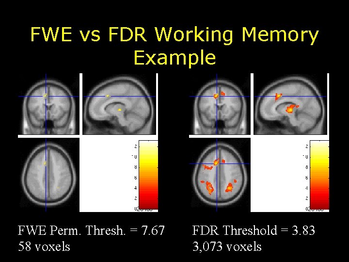
FWE vs FDR Working Memory Example FWE Perm. Thresh. = 7. 67 58 voxels FDR Threshold = 3. 83 3, 073 voxels

FDR Properties • Adaptive – Larger the signal, the lower the threshold – Larger the signal, the more false positives • False positives constant as fraction of rejected tests • Not much a problem with imaging’s sparse signals • Smoothing data very helpful – Smoothing introduces positive correlations

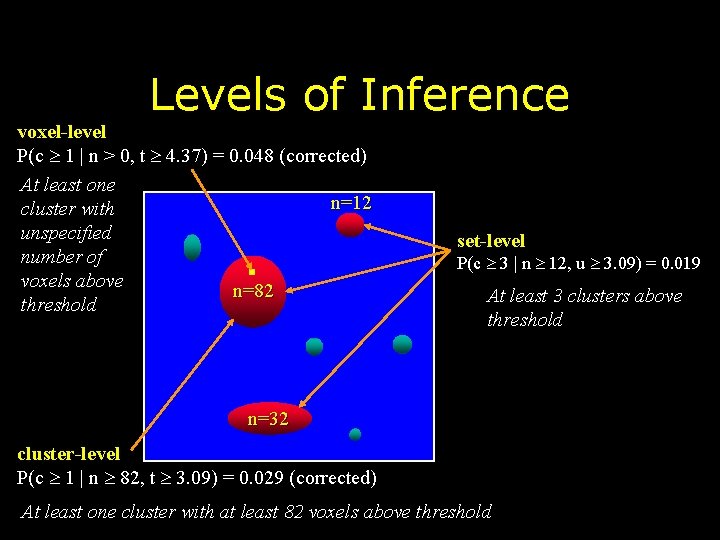
Levels of Inference voxel-level P(c 1 | n > 0, t 4. 37) = 0. 048 (corrected) At least one n=12 cluster with unspecified number of voxels above n=82 threshold set-level P(c 3 | n 12, u 3. 09) = 0. 019 At least 3 clusters above threshold n=32 cluster-level P(c 1 | n 82, t 3. 09) = 0. 029 (corrected) At least one cluster with at least 82 voxels above threshold

SPM Statistics Report • FWE-corr is the random field theory corrected p-value at the voxel level • FDR-corr is the false discovery rate corrected p -value at the voxel level • Cluster-level corrected p-value is RFT using both cluster size and maximum t-statistic

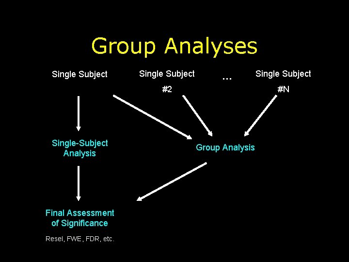
Group Analyses Single Subject … #2 Single-Subject Analysis Final Assessment of Significance Resel, FWE, FDR, etc. Single Subject #N Group Analysis

Within-Subject Analysis Observed f. MRI Time Series Observed – Fitted Boxcar S SE between-scan variability Fitted Boxcar t= S SE

Pool Data Across Subjects? • Perform single-subject analysis on each subject • Then show the results for each subject. Basically, present data as a collection of case reports • Does not provide any statistical significance to the results • If 8 out 10 subjects activate in an area is that significant?

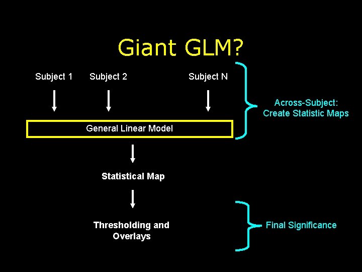
Giant GLM? Subject 1 Subject 2 Subject N Across-Subject: Create Statistic Maps General Linear Model Statistical Map Thresholding and Overlays Final Significance

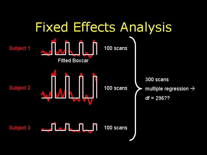
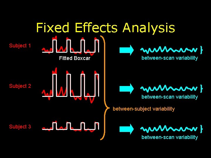
Fixed Effects Analysis Subject 1 100 scans Fitted Boxcar 300 scans Subject 2 100 scans multiple regression df = 296? ? Subject 3 100 scans

Fixed Effects Analysis Subject 1 Fitted Boxcar between-scan variability Subject 2 between-scan variability between-subject variability Subject 3 between-scan variability

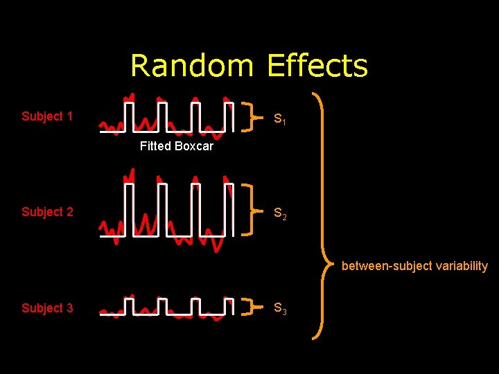
Random Effects Subject 1 S 1 Fitted Boxcar Subject 2 S 2 between-subject variability Subject 3 S 3

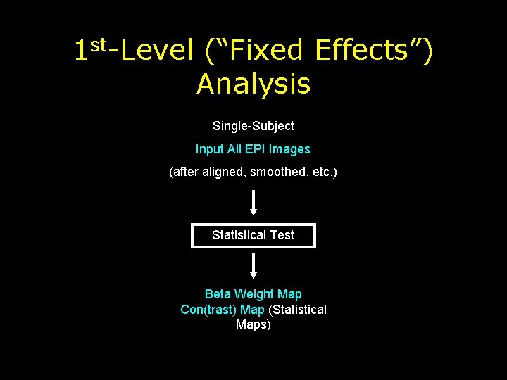
1 st-Level (“Fixed Effects”) Analysis Single-Subject Input All EPI Images (after aligned, smoothed, etc. ) Statistical Test Beta Weight Map Con(trast) Map (Statistical Maps)

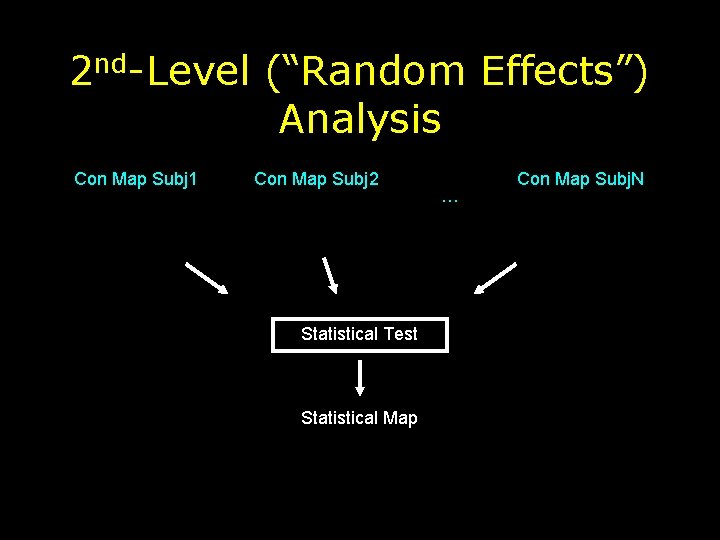
2 nd-Level (“Random Effects”) Analysis Con Map Subj 1 Con Map Subj 2 Statistical Test Statistical Map … Con Map Subj. N

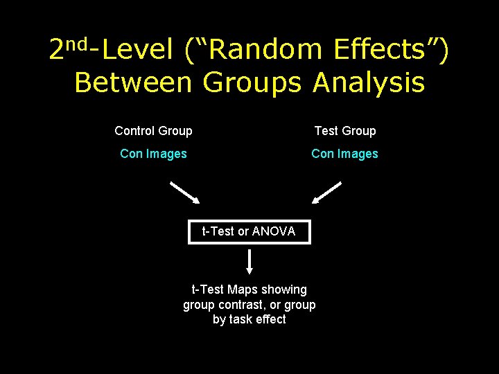
2 nd-Level (“Random Effects”) Between Groups Analysis Control Group Test Group Con Images t-Test or ANOVA t-Test Maps showing group contrast, or group by task effect

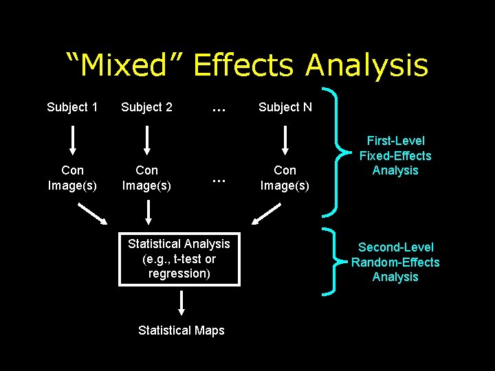
“Mixed” Effects Analysis Subject 1 Con Image(s) Subject 2 Con Image(s) … … Statistical Analysis (e. g. , t-test or regression) Statistical Maps Subject N Con Image(s) First-Level Fixed-Effects Analysis Second-Level Random-Effects Analysis

Random Effects Summary • Pool data across subjects • Inference generalizes to the population level • Both inter-subject and inter-scan variability properly accounted for

Data Driven Analysis Methods • All statistical approaches described so far use a model of our expectation of the activity (eg. on-off periodicity of the our block design, etc) • Data driven methods make no assumptions and instead use automated techniques to find changes of interest – Fourier Analysis – Independent Component Analysis (ICA) – Partial Least Squares (PLS) – Etc…

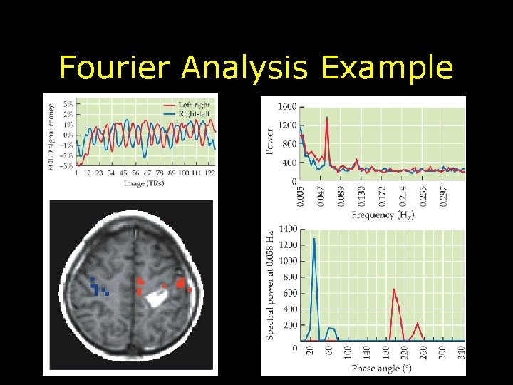
Fourier Analysis • Examines temporal structure of the f. MRI data • Analyzes f. MRI data in frequency domain which represents data as power for each frequency component • Note this has nothing to do with image reconstruction or k-space – Advantage: Makes no assumptions about the data – Disadvantage: Can only be used with block-design types of paradigms

Fourier Analysis Example

Independent Components Analysis (ICA) • Model-free (ie. data driven technique) • Computational method to decompose data into subcomponents that are mutually independent • When summed they represent the original signal • All voxels that match the pattern are picked up irregardless of spatial location