Statistics Objectives The students will be able to

+ Statistics Objectives: The students will be able to … 1. Identify and define a Normal Curve by its mean and standard deviation. 2. Use the 68 – 95 – 99. 7 Rule to calculate probabilities

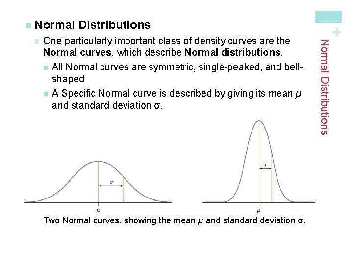
One particularly important class of density curves are the Normal curves, which describe Normal distributions. n All Normal curves are symmetric, single-peaked, and bellshaped n A Specific Normal curve is described by giving its mean µ and standard deviation σ. Two Normal curves, showing the mean µ and standard deviation σ. Normal Distributions n Distributions + n Normal

Definition: A Normal distribution is described by a Normal density curve. Any particular Normal distribution is completely specified by two numbers: its mean µ and standard deviation σ. • The mean of a Normal distribution is the center of the symmetric Normal curve. • The standard deviation is the distance from the center to the changeof-curvature points on either side. • We abbreviate the Normal distribution with mean µ and standard deviation σ as N(µ, σ). + Distributions Normal Distributions n Normal distributions are good descriptions for some distributions of real data. Normal distributions are good approximations of the results of many kinds of chance outcomes. Many statistical inference procedures are based on Normal distributions.

+ Normal Curve Applet n Now go to the Normal Curve applet bookmarked on my website at bchs. net. n n n Drag the two green dots at the top of the graph so that the mean of the curve is 0 and the standard deviation is 1. If you were to place the two green dots exactly one standard deviation on either side of the mean, what would the applet say is the area between them? If you were to place the two green dots exactly two standard deviations on either side of the mean, what would the applet say is the area between them? If you were to place the two green dots exactly three standard deviations on either side of the mean, what would the applet say is the are between them? To find the area between, click on “Show probability calculations”

+ Normal Curve Applet n Will changing the mean and standard deviation of the normal curve change the area that is between one, two, and three standard deviations from the mean? n Change n Find the area that is between one, two, and three standard deviations from the mean. n Change n the mean to 4 and the standard deviation to 0. 60. the mean to 3 and the standard deviation to 1. 5. What percent of the area under this normal density curve lies within one, two, and three standard deviations of the mean?

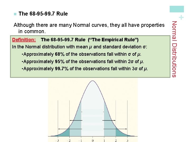
The 68 -95 -99. 7 Rule Definition: The 68 -95 -99. 7 Rule (“The Empirical Rule”) In the Normal distribution with mean µ and standard deviation σ: • Approximately 68% of the observations fall within σ of µ. • Approximately 95% of the observations fall within 2σ of µ. • Approximately 99. 7% of the observations fall within 3σ of µ. Normal Distributions Although there are many Normal curves, they all have properties in common. + n

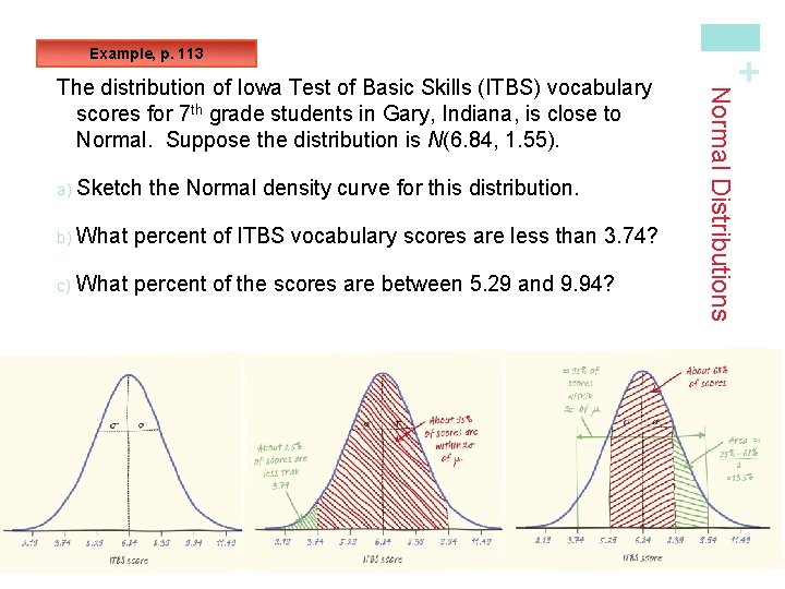
a) Sketch the Normal density curve for this distribution. b) What percent of ITBS vocabulary scores are less than 3. 74? c) What percent of the scores are between 5. 29 and 9. 94? Normal Distributions The distribution of Iowa Test of Basic Skills (ITBS) vocabulary scores for 7 th grade students in Gary, Indiana, is close to Normal. Suppose the distribution is N(6. 84, 1. 55). + Example, p. 113

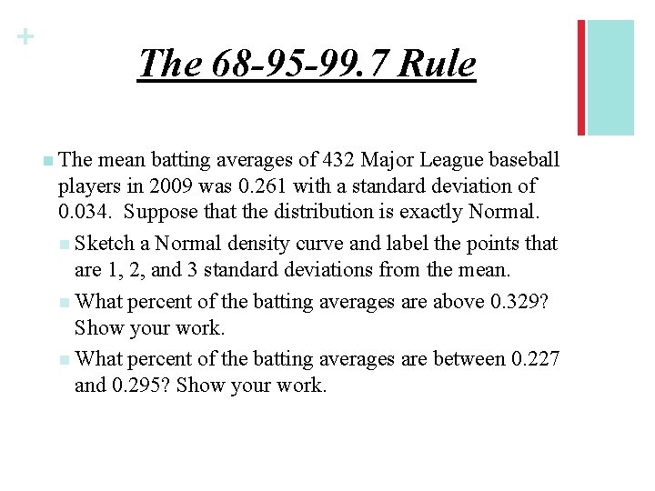
+ The 68 -95 -99. 7 Rule n The mean batting averages of 432 Major League baseball players in 2009 was 0. 261 with a standard deviation of 0. 034. Suppose that the distribution is exactly Normal. n Sketch a Normal density curve and label the points that are 1, 2, and 3 standard deviations from the mean. n What percent of the batting averages are above 0. 329? Show your work. n What percent of the batting averages are between 0. 227 and 0. 295? Show your work.

+ Homework n Page 131 (41 – 44)

+ Statistics Objectives: The students will be able to … 1. Find the area under a Normal curve using a Table. 2. Use the table to find the z-score for given percentiles.

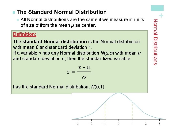
All Normal distributions are the same if we measure in units of size σ from the mean µ as center. Definition: The standard Normal distribution is the Normal distribution with mean 0 and standard deviation 1. If a variable x has any Normal distribution N(µ, σ) with mean µ and standard deviation σ, then the standardized variable has the standard Normal distribution, N(0, 1). Normal Distributions n Standard Normal Distribution + n The

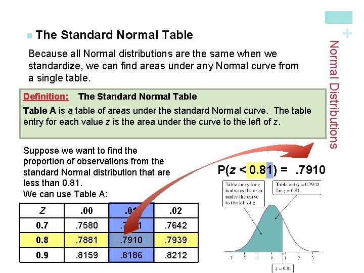
+ Standard Normal Table Because all Normal distributions are the same when we standardize, we can find areas under any Normal curve from a single table. Definition: The Standard Normal Table A is a table of areas under the standard Normal curve. The table entry for each value z is the area under the curve to the left of z. Suppose we want to find the proportion of observations from the standard Normal distribution that are less than 0. 81. We can use Table A: Z . 00 . 01 . 02 0. 7 . 7580 . 7611 . 7642 0. 8 . 7881 . 7910 . 7939 0. 9 . 8159 . 8186 . 8212 P(z < 0. 81) =. 7910 Normal Distributions n The

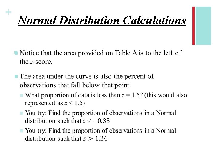
+ Normal Distribution Calculations n

+ Normal Distribution Calculations n Common Mistake! Reporting the entry for the corresponding z – value, regardless of whether the problem asks for the area to the left or to the right of that z – value. n How to avoid? Always sketch the Normal curve, mark the z – value, and shade the area of interest. Then make sure your answer is reasonable in the context of the problem.

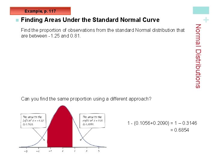
Example, p. 117 Finding Areas Under the Standard Normal Curve Normal Distributions Find the proportion of observations from the standard Normal distribution that are between -1. 25 and 0. 81. + n Can you find the same proportion using a different approach? 1 - (0. 1056+0. 2090) = 1 – 0. 3146 = 0. 6854

+ Normal Distribution Calculations n Sketch the curve and shade the area of interest. Then, Find the proportion of observations that fall between -0. 58 and 1. 79. n Find the proportion of observations that fall between 0. 24 and 1. 24. n

+ Normal Distribution Calculations n The table can also be used backwards. n Meaning, if I give you the area under the curve, can you find the z-score that corresponds to that area? Find the z-score that corresponds to the 25 th percentile. n Find the point so that 60% of all observations are greater than z. n n You still want to sketch a curve and shade the area of interest.

+ Homework n. Page 131 (47 – 52)

+ Normal Distribution Calculations n The command normalpdf gives the height of a Normal curve for a particular value if x, mean μ, and standard deviation σ. For example, normalpdf (0, 0, 1) = 0. 3989 gives the height of the standard Normal curve at its peak. n What if we reverse the process? What z – score corresponds to the 90 th percentile? n The inv. Norm function can do this. n Enter inv. Norm (percentile, μ, σ)

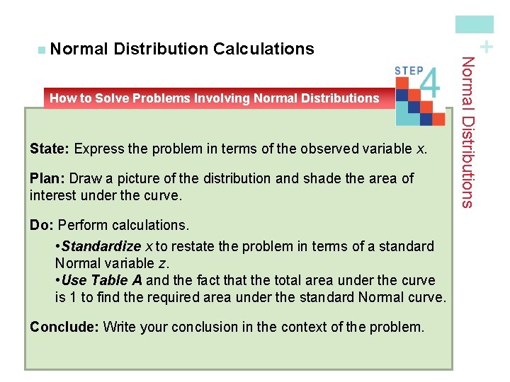
How to Solve Problems Involving Normal Distributions State: Express the problem in terms of the observed variable x. Plan: Draw a picture of the distribution and shade the area of interest under the curve. Do: Perform calculations. • Standardize x to restate the problem in terms of a standard Normal variable z. • Use Table A and the fact that the total area under the curve is 1 to find the required area under the standard Normal curve. Conclude: Write your conclusion in the context of the problem. + Distribution Calculations Normal Distributions n Normal

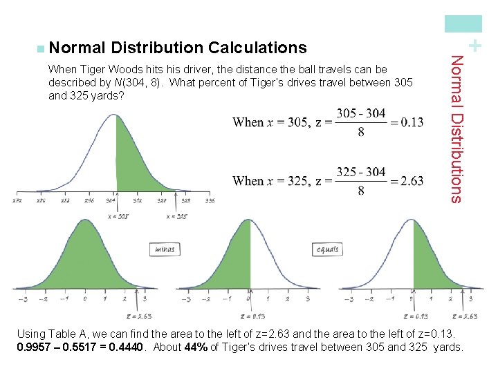
When Tiger Woods hits his driver, the distance the ball travels can be described by N(304, 8). What percent of Tiger’s drives travel between 305 and 325 yards? + Distribution Calculations Normal Distributions n Normal Using Table A, we can find the area to the left of z=2. 63 and the area to the left of z=0. 13. 0. 9957 – 0. 5517 = 0. 4440. About 44% of Tiger’s drives travel between 305 and 325 yards.

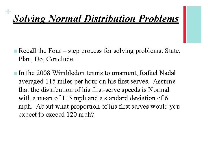
+ Solving Normal Distribution Problems n Recall the Four – step process for solving problems: State, Plan, Do, Conclude n In the 2008 Wimbledon tennis tournament, Rafael Nadal averaged 115 miles per hour on his first serves. Assume that the distribution of his first-serve speeds is Normal with a mean of 115 mph and a standard deviation of 6 mph. About what proportion of his first serves would you expect to exceed 120 mph?

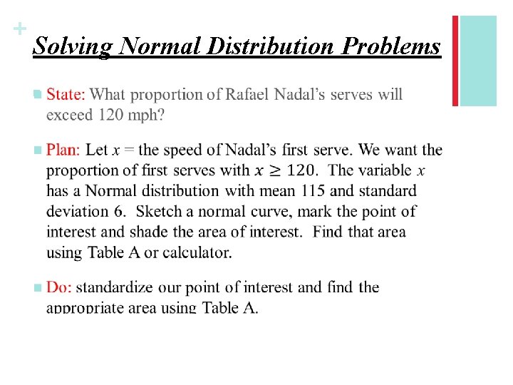
+ Solving Normal Distribution Problems n

+ Solving Normal Distribution Problems n What percent of Rafael Nadal’s first serves are between 100 and 110 mph? n State, Plan, Do, Conclude n What is the third quartile of Rafael Nadal’s first serves? n State, Plan, Do, Conclude

+ Homework n. Page 132 (53, 55, 57, 59, 61)