Statistics in MSmc DESPOT Jason Su borrowed heavily

Statistics in MSmc. DESPOT Jason Su (borrowed heavily from STATS 191 and Prof. Jonathan Taylor)

Comparison of 2 Populations • Null hypothesis (H 0): The populations are the same • Alternative hypothesis (HA): The populations are different. • t-test is the standard tool used here – Assumes the two populations are Gaussian distributed but that the data follows a t-dist. since we must estimate the mean and standard deviation • Wilcoxon rank-sum (or Mann–Whitney U) test – Is a non-parametric version, does not assume a distribution – Compares the medians instead of means of population • Reject at p-value < 0. 05 level typically. – Interpretation: assuming the null hypothesis the p-value is the chance that we would observe something as extreme as the 2 nd sample – Rejection at 0. 05, means we would tolerate being wrong 5% of the time if they are actually the same

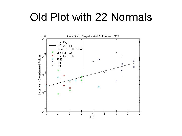
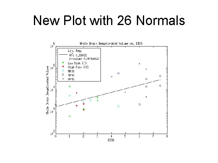
Simple Linear Regression • y = a*x + b • Least squares fit of the predictor to the outcome, equiv. to maximum likelihood if assumptions correct – Assumptions: full column rank, residuals are independent N(0, σ^2) constant variance – In MSmc. DESPOT predictor is log(DV), outcome is EDSS – EDSS = a*log(DV) + b • R^2 is a measure of how much of the variability of the outcome is explained by the predictor

Diagnostics • What can go wrong? – Wrong regression function – Incorrect model for errors • Not normal • Not independent • Non-constant variance • Tools – Q-Q Plot, plot the quantiles of the residuals vs. that of a normal, should be a linear relationship – Plot residuals vs. predictor

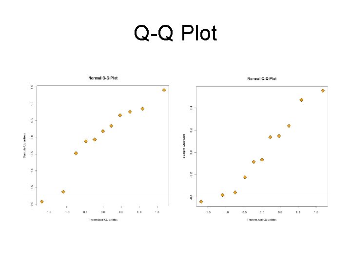
Q-Q Plot

Non-constant Variance

Multiple Linear Regression • Y = X*a – a = pinv(X)*Y, LS solution, pinv(X) = inv(X’X)X’ – X is now a matrix of columns of predictors • The outcome is linear in a predictor after accounting for all the others • Same assumptions from simple lin. reg. also • Adding even random noise to X improves R^2 – Adjusted R^2, instead of sum of square error, use mean square error: favors simpler models

Diagnostics • Old tools are still good • New tools to measure the influence of an observation, useful for determining outliers – DFFITS: measures how much the regression function changes at the i-th observation when the i-th row is removed from X – Cook’s distance: how much the entire regression function changes when i-th row removed – DFBETAS: how much coefficients change when i-th row removed

Model Selection • As suggested by Adjusted R^2, what we really want is a parsimonious model – One that predicts the outcome well with only a few predictors • This is a combinatorially hard problem • Models are evaluated with a criterion – – – Adjusted R^2 Mallow’s Cp – estimated predictive power of model Akaike information criterion (AIC) – related to Cp Bayesian information criterion (BIC) Cross validation with MSE

Search Strategy • If the model is small enough, can search all – In MSmc. DESPOT this is probably feasible, our predictors are: age, PVF, log(DV), gender, PP, SP, RR, CIS – 127 possibilities • Stepwise – This is a popular search method where the algorithm is giving a starting point then adds or removes predictors one at a time until there is no improvement in the criterion

New Results with All 26 Normals

Old Plot with 22 Normals

New Plot with 26 Normals

Discussion • All the relevant rank sum tests (Normals vs. classes of MS, RR vs. SP) are still below the p < 0. 01 threshold as before • The drop in correlation is probably due to N 024, who shows an unusually high amount of demyelination at half the level of the lowest CIS patients, could be an outlier • I’m not certain if log() is the correct transform for DV, need to run more diagnostics • How accurate is EDSS?

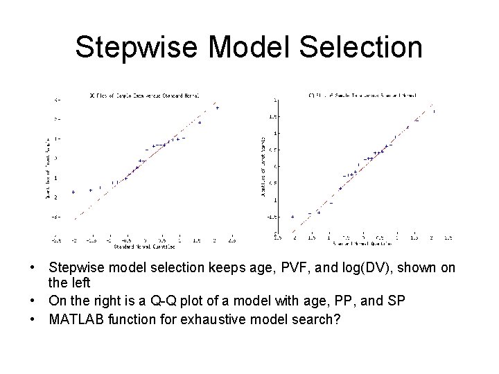
Stepwise Model Selection • Stepwise model selection keeps age, PVF, and log(DV), shown on the left • On the right is a Q-Q plot of a model with age, PP, and SP • MATLAB function for exhaustive model search?