STATISTICS IN GEOGRAPHY USING STATISTICS TO DESCRIBE GEOGRAPHICAL
STATISTICS IN GEOGRAPHY USING STATISTICS TO DESCRIBE GEOGRAPHICAL DATA
During a GEOGRAPHICAL INVESTIGATION there is a set sequence of events: - • Decide on the area of investigation and do some background research so that you are aware of the main ideas, concepts and factors involved. • Formulate a hypothesis based on the information you have researched. • Decide what data you will need to collect to test your idea / ideas, and produce a data collection plan involving data collection / sampling methods. Collect the data. • Classify the data, begin the statistical analysis and present the data with appropriate maps, graphs and images. • Analyse and Interpret the data, reach substantiated conclusions (related to your hypothesis / hypotheses) and discuss the effectiveness and limitations of the study. This powerpoint is about the classification and statistical analysis of data.
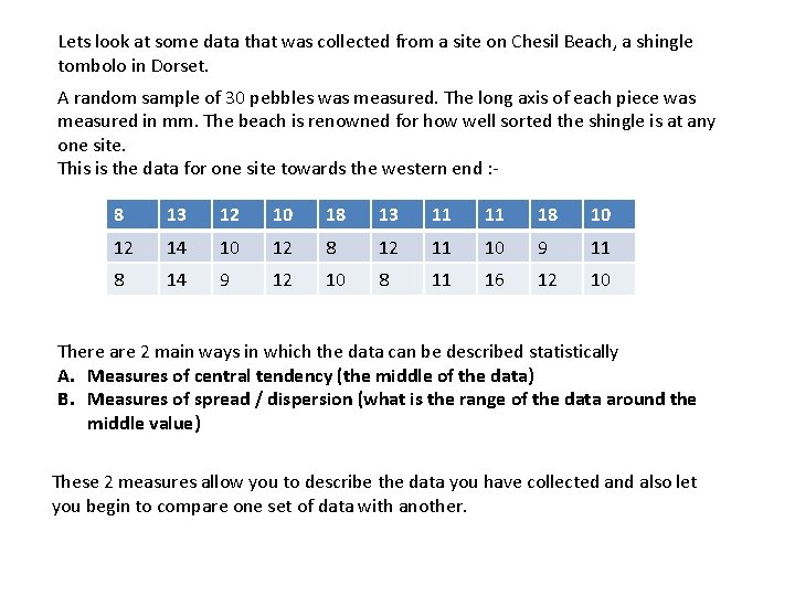
Lets look at some data that was collected from a site on Chesil Beach, a shingle tombolo in Dorset. A random sample of 30 pebbles was measured. The long axis of each piece was measured in mm. The beach is renowned for how well sorted the shingle is at any one site. This is the data for one site towards the western end : 8 13 12 10 18 13 11 11 18 10 12 14 10 12 8 12 11 10 9 11 8 14 9 12 10 8 11 16 12 10 There are 2 main ways in which the data can be described statistically A. Measures of central tendency (the middle of the data) B. Measures of spread / dispersion (what is the range of the data around the middle value) These 2 measures allow you to describe the data you have collected and also let you begin to compare one set of data with another.
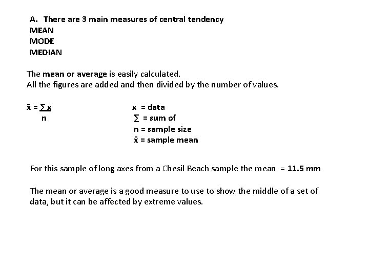
A. There are 3 main measures of central tendency MEAN MODE MEDIAN The mean or average is easily calculated. All the figures are added and then divided by the number of values. x = ∑ x n x = data ∑ = sum of n = sample size x = sample mean For this sample of long axes from a Chesil Beach sample the mean = 11. 5 mm The mean or average is a good measure to use to show the middle of a set of data, but it can be affected by extreme values.
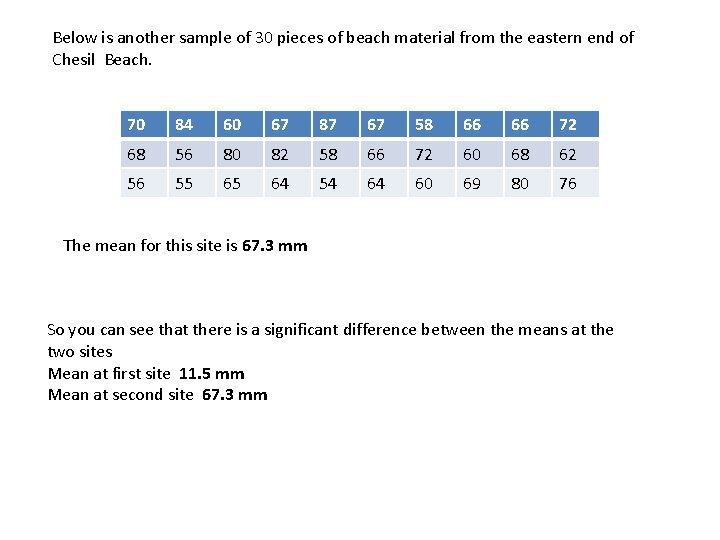
Below is another sample of 30 pieces of beach material from the eastern end of Chesil Beach. 70 84 60 67 87 67 58 66 66 72 68 56 80 82 58 66 72 60 68 62 56 55 65 64 54 64 60 69 80 76 The mean for this site is 67. 3 mm So you can see that there is a significant difference between the means at the two sites Mean at first site 11. 5 mm Mean at second site 67. 3 mm
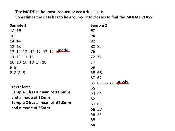
The MODE is the most frequently occurring value. Sometimes the data has to be grouped into classes to find the MODAL CLASS Sample 1 18 18 16 14 14 13 13 12 12 mode 11 11 10 10 10 9 9 8 8 Therefore: Sample 1 has a mean of 11. 5 mm and a mode of 12 mm Sample 2 has a mean of 67. 3 mm and a mode of 66 mm Sample 2 87 84 82 80 80 76 72 72 70 69 68 68 67 67 66 66 mode 65 64 64 62 60 60 58 58 56 56 55 54
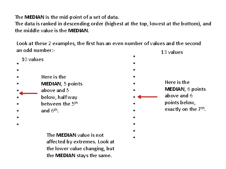
The MEDIAN is the mid-point of a set of data. The data is ranked in descending order (highest at the top, lowest at the bottom), and the middle value is the MEDIAN. Look at these 2 examples, the first has an even number of values and the second an odd number: 13 values * 10 values * * Here is the MEDIAN, 5 points * * MEDIAN, 6 points above and 5 * * above and 6 below, half way * * points below, between the 5 th * * exactly on the 7 th. and 6 th. * * * * The MEDIAN value is not * affected by extremes. Look at the lower value changing, but the MEDIAN stays the same.
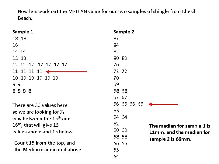
Now lets work out the MEDIAN value for our two samples of shingle from Chesil Beach. Sample 1 18 18 16 14 14 13 13 12 12 11 11 10 10 10 9 9 8 8 There are 30 values here so we are looking for ½ way between the 15 th and 16 th, that will give 15 values above and 15 below Count 15 from the top, and the Median is indicated above Sample 2 87 84 82 80 80 76 72 72 70 69 68 68 67 67 66 66 65 64 64 62 60 60 58 58 56 56 55 54 The median for sample 1 is 11 mm, and the median for sample 2 is 66 mm.
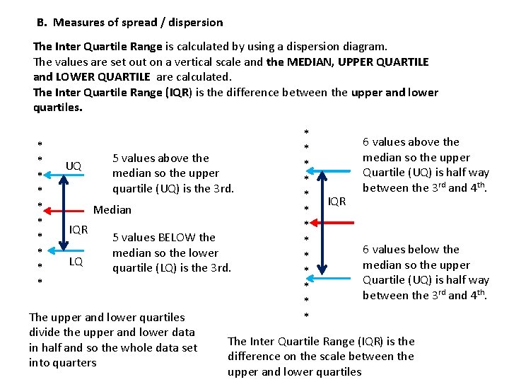
B. Measures of spread / dispersion The Inter Quartile Range is calculated by using a dispersion diagram. The values are set out on a vertical scale and the MEDIAN, UPPER QUARTILE and LOWER QUARTILE are calculated. The Inter Quartile Range (IQR) is the difference between the upper and lower quartiles. * * * * * UQ 5 values above the median so the upper quartile (UQ) is the 3 rd. Median IQR LQ 5 values BELOW the median so the lower quartile (LQ) is the 3 rd. The upper and lower quartiles divide the upper and lower data in half and so the whole data set into quarters * * * * IQR 6 values above the median so the upper Quartile (UQ) is half way between the 3 rd and 4 th. 6 values below the median so the upper Quartile (UQ) is half way between the 3 rd and 4 th. The Inter Quartile Range (IQR) is the difference on the scale between the upper and lower quartiles
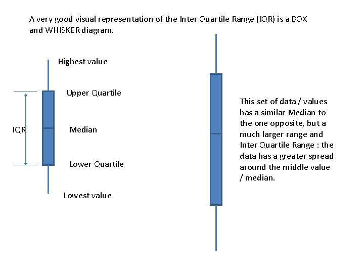
A very good visual representation of the Inter Quartile Range (IQR) is a BOX and WHISKER diagram. Highest value Upper Quartile IQR Median Lower Quartile Lowest value This set of data / values has a similar Median to the one opposite, but a much larger range and Inter Quartile Range : the data has a greater spread around the middle value / median.
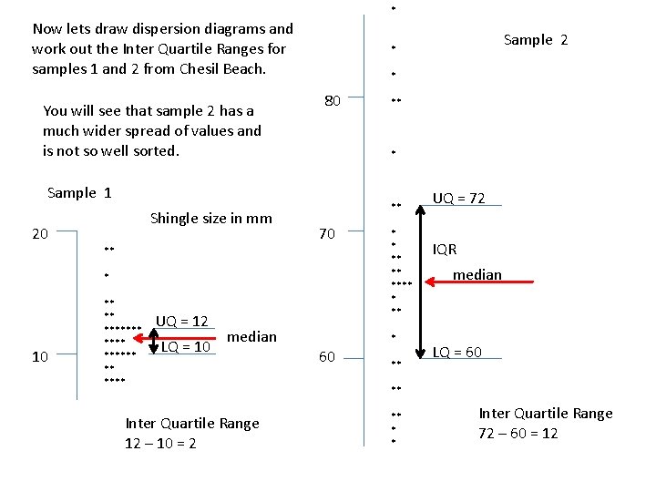
* Now lets draw dispersion diagrams and work out the Inter Quartile Ranges for samples 1 and 2 from Chesil Beach. You will see that sample 2 has a much wider spread of values and is not so well sorted. * 80 20 ** 70 ** * 10 ** ** ******* ** **** UQ = 12 LQ = 10 median Inter Quartile Range 12 – 10 = 2 ** * Sample 1 Shingle size in mm Sample 2 * ** ** **** * 60 ** UQ = 72 IQR median LQ = 60 ** ** * * Inter Quartile Range 72 – 60 = 12
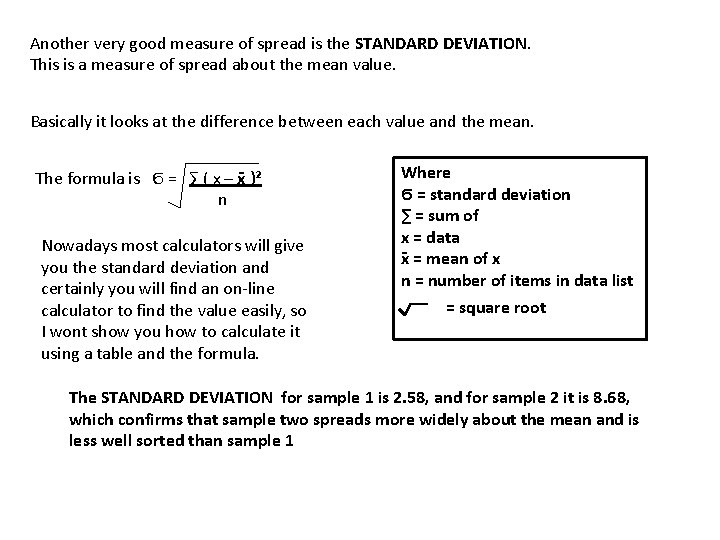
Another very good measure of spread is the STANDARD DEVIATION. This is a measure of spread about the mean value. Basically it looks at the difference between each value and the mean. The formula is Ϭ = ∑ ( x – x )² n Nowadays most calculators will give you the standard deviation and certainly you will find an on-line calculator to find the value easily, so I wont show you how to calculate it using a table and the formula. Where Ϭ = standard deviation ∑ = sum of x = data x = mean of x n = number of items in data list = square root The STANDARD DEVIATION for sample 1 is 2. 58, and for sample 2 it is 8. 68, which confirms that sample two spreads more widely about the mean and is less well sorted than sample 1
- Slides: 12