Statistics for Microarrays Linear and Nonlinear Modeling Class

Statistics for Microarrays Linear and Nonlinear Modeling Class web site: http: //statwww. epfl. ch/davison/teaching/Microarrays/

c. DNA gene expression data Data on G genes for n samples m. RNA samples sample 1 sample 2 sample 3 sample 4 sample 5 … Genes 1 2 3 4 5 0. 46 -0. 10 0. 15 -0. 45 -0. 06 0. 30 0. 49 0. 74 -1. 03 1. 06 0. 80 0. 24 0. 04 -0. 79 1. 35 1. 51 0. 06 0. 10 -0. 56 1. 09 0. 90 0. 46 0. 20 -0. 32 -1. 09 . . . . Gene expression level of gene i in m. RNA sample j = (normalized) Log( Red intensity / Green intensity)

Identifying Differentially Expressed Genes • Goal: Identify genes associated with covariate or response of interest • Examples: – Qualitative covariates or factors: treatment, cell type, tumor class – Quantitative covariate: dose, time – Responses: survival, cholesterol level – Any combination of these!

Modeling Introduction • Want to capture important features of the relationship between a (set of) variable(s) and one or more responses • Many models are of the form g(Y) = f(x) + error • Differences in the form of g, f and distributional assumptions about the error term

Examples of Models • Linear: Y = 0 + 1 x + 2 x 2 + • (Intrinsically) Nonlinear: Y = x 1 x 2 x 3 + • Generalized Linear Model (e. g. Binomial): ln(p/[1 -p]) = 0 + 1 x 1 + 2 x 2 • Proportional Hazards (in Survival Analysis): h(t) = h 0(t) exp( x)

Linear Modeling • A simple linear model: E(Y) = 0 + 1 x • Gaussian measurement model: Y = 0 + 1 x + , where ~ N(0, 2) • More generally: Y = X + , where Y is n x 1, X is n x G, is G x 1, is n x 1, often assumed N(0, 2 Inxn)

Analysis of Designed Experiments • An important use of linear models • Here, the response (Y) is the gene expression level • Define a (design) matrix X so that E(Y) = X , where is a vector of contrasts • Many ways to define design matrix/contrasts

Contrasts (I) • Example: One-way layout, k classes Yij = + j + ij, i = 1, …, nj; j = 1, …, k X = 1 1 0 … 0 = [1 Xa] 101… 0 … 100… 1 • Problem: this specification is overparametrized

Contrasts (II) • Could resolve by removing column of 1’s: Yij = j + ij, i = 1, …, nj; j = 1, …, k X = 1 0 … 0 = [Xa] 01… 0 … 00… 1 • Here, parameters are class means

Contrasts (III) • Define design matrix X* = [1 Xa. Ca], with Ca (k x (k-1)) chosen so that X* has rank k (the number of columns) • Parameters may become difficult to interpret • In the balanced case (equal number of observations in each class), can choose orthogonal contrasts (Helmert)

Model Fitting • For the standard (fixed effects) linear model, estimation is usually by least squares • Can be more complicated with random effects or when x-variables subject to measurement error as well (so that estimates are not biased)

Model Checking • Examination of residuals – – Normality Time effects Nonconstant variance Curvature • Detection of influential observations

Do we need robust methods? • Tukey (1962): “A tacit hope in ignoring deviations from ideal models was that they would not matter; that statistical procedures which were optimal under the strict model would still be approximately optimal under the approximate model. Unfortunately it turned out that this hope was often drastically wrong; even mild deviations often have much larger effects than were anticipated by most statisticians. ”

Robust Regression • Idea: downweight observations that produce large residuals • More computationally intensive than least squares regression (which gives equal weight to each observation) • Use maximum likelihood if can assume specific error distribution • When not, use M-estimators

M-estimators • ‘Maximum likelihood type’ estimators • Assume independent errors with distribution f( ) • Robust estimator minimizes i (ei/s) = i {(Yi – xi’ )/s}, where (. ) is some function and s is an estimate of scale • (u) = u 2 corresponds to minimizing the sum of squares

M-estimation Procedure • To minimize i {(Yi – xi’ )/s} wrt the ’s, take derivatives and equate to 0 • Resulting equations do not have an explicit solution in general • Solve by iteratively reweighted least squares

Examples of Weight Functions

Generalized Linear Models (GLM/GLIM) • Response Y assumed to have exponential family distribution: f(y) = exp[a(y)b( ) + c( ) + d(y)] • Parameters and explanatory variables X; linear predictor = 1 x 1 + 2 x 2 + … pxp • Mean response , link function l ( ) = • Allows unified treatment of statistical methods for several important classes of models

Some Examples Link logit probit cloglog identity inverse Log Sqrt Binomial Default X X Gamma Normal Poisson X X Default X

(BREAK)

Survival Modeling • Response T is a (nonnegative) lifetime • Cumulative distribution function (cdf) F(t), density f(t) • More usual to work with the survivor function S(t) = 1 – F(t) = P(T > t) and the instantaneous failure rate, or hazard function h(t) = lim t->0 P(t T< t+ t | T t)/ t

Relations Between Functions • Cumulative hazard function H(t) = 0 t h(s) ds • h(t) = f(t)/S(t) • H(t) = -log S(t)

Censoring • Incomplete information on the lifetime • A censored observation is one whose value is incomplete due to random factors for each individual • Most commonly, observation begins at time t = 0 and ends before the outcome of interest is observed (right-censoring)

Estimation of Survivor Function • Most commonly used estimate is Kaplan-Meier (also called product limit) estimator • Risk set r(t) = number of cases alive just before time t ^ • S(t) = ti t [r(ti) – di]/r(ti)

Cox Proportional Hazards Model • Baseline hazard function h 0(t) • Modified multiplicatively by covariates • Hazard function for individual case is h(t) = h 0(t) exp( 1 x 1 + 2 x 2 + … + pxp) • If nonproportionality: – 1. Does it matter – 2. Is it real

Strategies for Gene Expression-based Modeling • The biggest problem is the large number of variables (genes) • One possibility is to first reduce the number of genes under consideration (e. g. consider variability across samples, or coefficient of variation) • Screening/Prioritizing: One gene at a time approach • Two at a time, perhaps plus interaction

Example: Survival analysis with expression data • Bittner et al. dataset: – 15 of the 31 melanomas had associated survival times – 3613 ‘strongly detected’ genes

Average Linkage Hierarchical Clustering unclustered ‘cluster’

Association of Variables • Variables tested for association with cluster: – Sex (p =. 68, n = 16 + 11 = 27) v. Age (p =. 14, n = 15 + 10 = 25) v. Mutation status (p =. 17, n = 12 + 7 = 19) – Biopsy site (p =. 88, n = 14 + 10 = 24) – Pigment (p =. 26, n = 13 + 9 = 22) – Breslow thickness (p =. 26, n = 6 + 3 = 9) – Clark level (p =. 44, n = 6 + 5 = 11) v. Specimen type (p =. 11, n = 11 + 12 = 23)

Survival analysis: Bittner et al. • Bittner et al. also looked at differences in survival between the two groups (the ‘cluster’ and the ‘unclustered’ samples) • ‘Cluster’ seemed associated with longer survival

Kaplan-Meier Survival Curves

Average Linkage Hierarchical Clustering, survival samples only unclustered cluster

Kaplan-Meier Survival Curves, new grouping

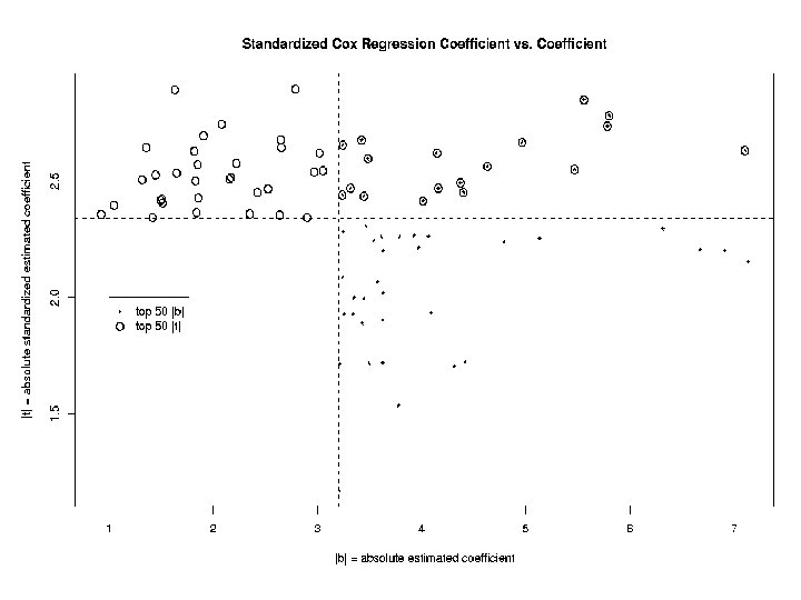
Identification of Genes Associated with Survival For each gene j, j = 1, …, 3613, model the instantaneous failure rate, or hazard function, h(t) with the Cox proportional hazards model: h(t) = h 0(t) exp( jxij) and look for genes with both: ^ • large effect size j ^ ^ • large standardized effect size j/SE( j)

Sites Potentially Influencing Survival Image Uni. Gene Cluster Title Clone ID Cluster 137209 Hs. 126076 Glutamate receptor interacting protein 240367 Hs. 57419 Transcriptional repressor 838568 825470 841501 Hs. 74649 Cytochrome c oxidase subunit Vlc Hs. 247165 ESTs, Highly similar to topoisomerase Hs. 77665 KIAA 0102 gene product

Findings • Top 5 genes by this method not in Bittner et al. ‘weighted gene list’ - Why? • weighted gene list based on entire sample; our method only used half • weighting relies on Bittner et al. cluster assignment • other possibilities?

Statistical Significance of Cox Model Coefficients

Advantages of Modeling • Can address questions of interest directly – Contrast with what has become the ‘usual’ (and indirect) approach with microarrays: clustering, followed by tests of association between cluster group and variables of interest • Great deal of existing machinery • Quantitatively assess strength of evidence

Limitations of Single Gene Tests • May be too noisy in general to show much • Do not reveal coordinated effects of positively correlated genes • Hard to relate to pathways

Not Covered… • Careful followup – Assessment of proportionality – Inclusion of combinations of genes, interactions – Consideration of alternative models • Power assessment – Not worth it here, there can’t be much!

Some ideas for further work • Expand models to include more genes, possibly two-way interactions – Issue of automation – Still very small scale compared to probable pathway size, number of genes involved, etc. • Nonparametric tree-based modeling – Will require much larger sample sizes

Acknowledgements • Debashis Ghosh • Erin Conlon • Sandrine Dudoit • José Correa