Statistics for Managers Using Microsoft Excel 5 th

Statistics for Managers Using Microsoft® Excel 5 th Edition Chapter 17 Decision Making Statistics for Managers Using Microsoft Excel, 5 e © 2008 Prentice-Hall, Inc. Chap 17 -1

Learning Objectives In this chapter, you learn: § To use payoff tables and decision trees to evaluate alternative courses of action § To use several criteria to select an alternative course of action § To use Bayes’ theorem to revise probabilities in light of sample information § About the concept of utility Statistics for Managers Using Microsoft Excel, 5 e © 2008 Prentice-Hall, Inc. 2

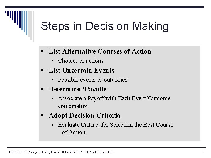
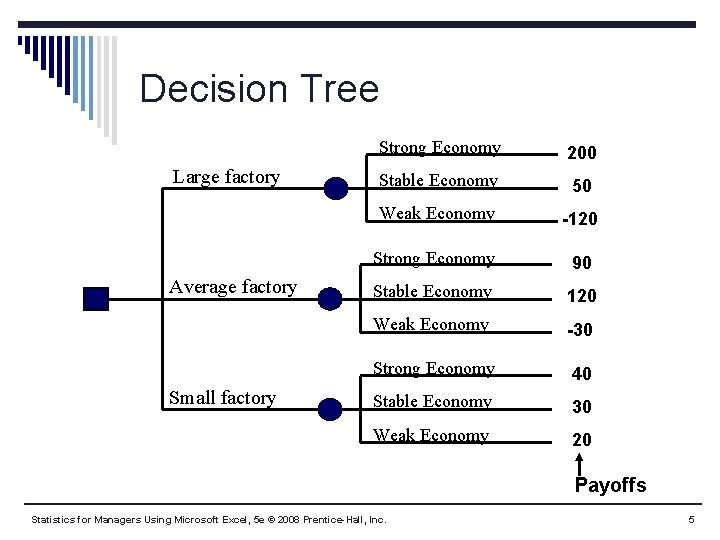
Steps in Decision Making § List Alternative Courses of Action § Choices or actions § List Uncertain Events § Possible events or outcomes § Determine ‘Payoffs’ § Associate a Payoff with Each Event/Outcome combination § Adopt Decision Criteria § Evaluate Criteria for Selecting the Best Course of Action Statistics for Managers Using Microsoft Excel, 5 e © 2008 Prentice-Hall, Inc. 3

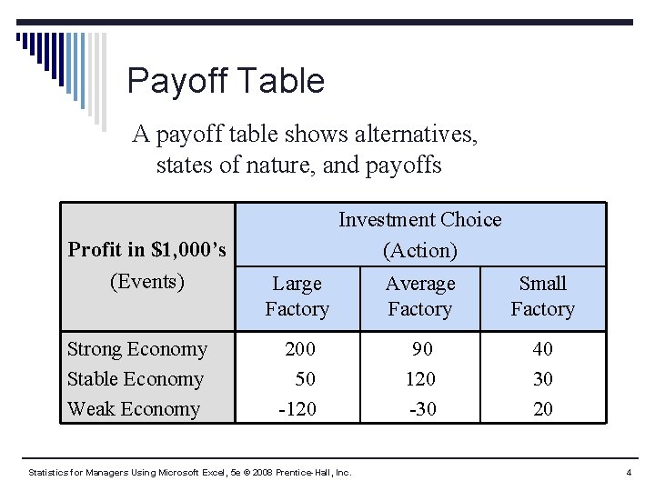
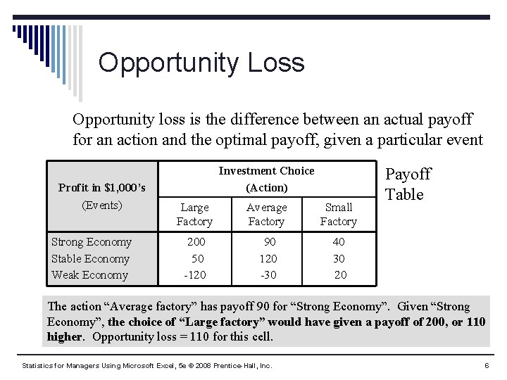
Payoff Table A payoff table shows alternatives, states of nature, and payoffs Profit in $1, 000’s (Events) Strong Economy Stable Economy Weak Economy Investment Choice (Action) Large Average Small Factory 200 50 -120 Statistics for Managers Using Microsoft Excel, 5 e © 2008 Prentice-Hall, Inc. 90 120 -30 40 30 20 4

Decision Tree Large factory Average factory Small factory Strong Economy 200 Stable Economy 50 Weak Economy -120 Strong Economy 90 Stable Economy 120 Weak Economy -30 Strong Economy 40 Stable Economy 30 Weak Economy 20 Payoffs Statistics for Managers Using Microsoft Excel, 5 e © 2008 Prentice-Hall, Inc. 5

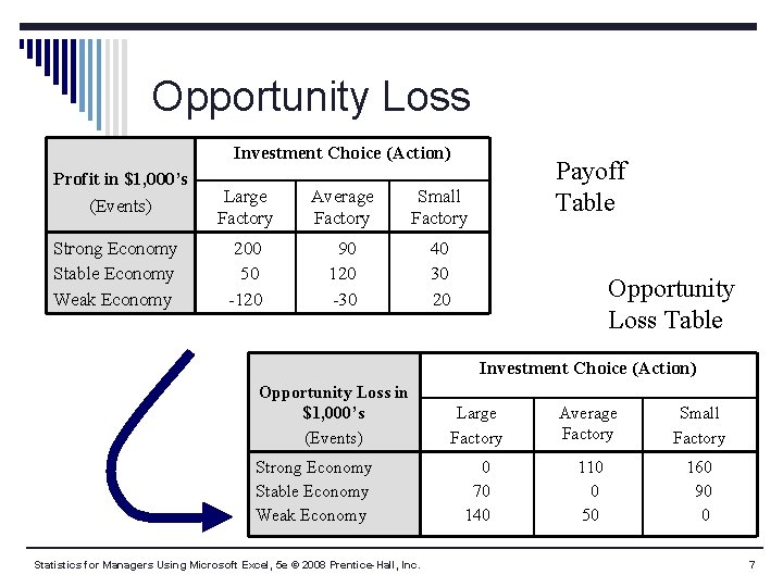
Opportunity Loss Opportunity loss is the difference between an actual payoff for an action and the optimal payoff, given a particular event Profit in $1, 000’s (Events) Strong Economy Stable Economy Weak Economy Investment Choice (Action) Large Factory Average Factory Small Factory 200 50 -120 90 120 -30 40 30 20 Payoff Table The action “Average factory” has payoff 90 for “Strong Economy”. Given “Strong Economy”, the choice of “Large factory” would have given a payoff of 200, or 110 higher. Opportunity loss = 110 for this cell. Statistics for Managers Using Microsoft Excel, 5 e © 2008 Prentice-Hall, Inc. 6

Opportunity Loss Investment Choice (Action) Profit in $1, 000’s (Events) Strong Economy Stable Economy Weak Economy Large Factory Average Factory Small Factory 200 50 -120 90 120 -30 40 30 20 Payoff Table Opportunity Loss Table Investment Choice (Action) Opportunity Loss in $1, 000’s (Events) Strong Economy Stable Economy Weak Economy Statistics for Managers Using Microsoft Excel, 5 e © 2008 Prentice-Hall, Inc. Large Factory Average Factory Small Factory 0 70 140 110 0 50 160 90 0 7

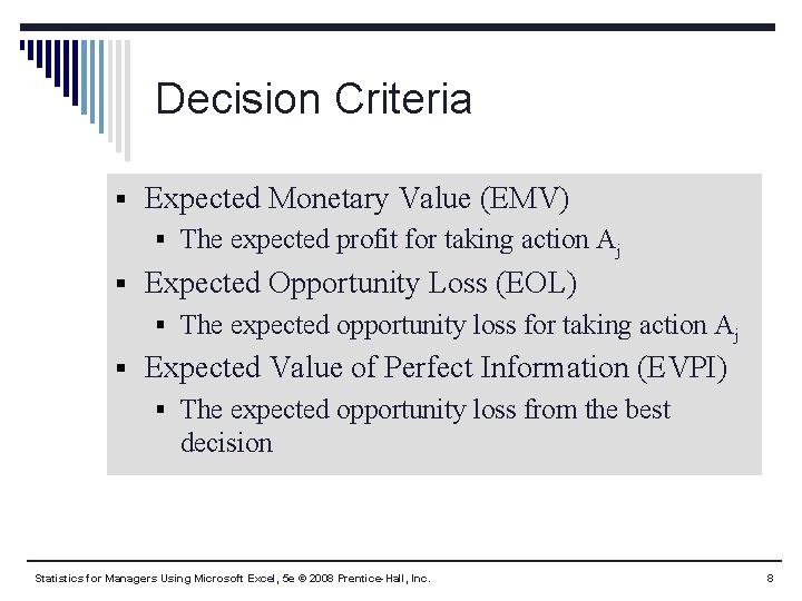
Decision Criteria § Expected Monetary Value (EMV) § The expected profit for taking action Aj § Expected Opportunity Loss (EOL) § The expected opportunity loss for taking action Aj § Expected Value of Perfect Information (EVPI) § The expected opportunity loss from the best decision Statistics for Managers Using Microsoft Excel, 5 e © 2008 Prentice-Hall, Inc. 8

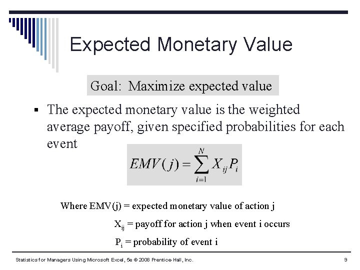
Expected Monetary Value Goal: Maximize expected value § The expected monetary value is the weighted average payoff, given specified probabilities for each event Where EMV(j) = expected monetary value of action j Xij = payoff for action j when event i occurs Pi = probability of event i Statistics for Managers Using Microsoft Excel, 5 e © 2008 Prentice-Hall, Inc. 9

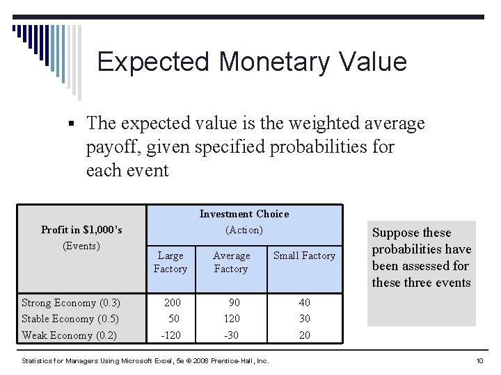
Expected Monetary Value § The expected value is the weighted average payoff, given specified probabilities for each event Profit in $1, 000’s (Events) Strong Economy (0. 3) Stable Economy (0. 5) Weak Economy (0. 2) Investment Choice (Action) Large Factory Average Factory Small Factory 200 50 -120 90 120 -30 40 30 20 Statistics for Managers Using Microsoft Excel, 5 e © 2008 Prentice-Hall, Inc. Suppose these probabilities have been assessed for these three events 10

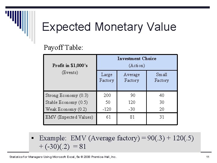
Expected Monetary Value Payoff Table: Profit in $1, 000’s (Events) Strong Economy (0. 3) Stable Economy (0. 5) Weak Economy (0. 2) EMV (Expected Values) Investment Choice (Action) Large Factory Average Factory Small Factory 200 50 -120 90 120 -30 40 30 20 61 81 31 § Example: EMV (Average factory) = 90(. 3) + 120(. 5) + (-30)(. 2) = 81 Statistics for Managers Using Microsoft Excel, 5 e © 2008 Prentice-Hall, Inc. 11

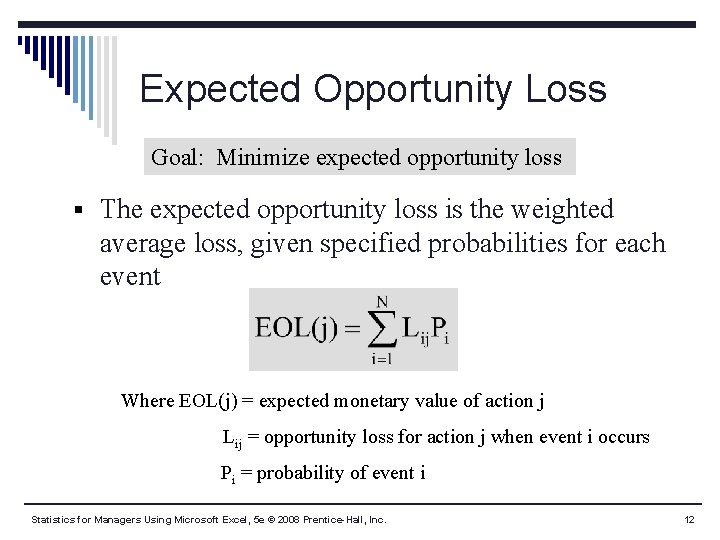
Expected Opportunity Loss Goal: Minimize expected opportunity loss § The expected opportunity loss is the weighted average loss, given specified probabilities for each event Where EOL(j) = expected monetary value of action j Lij = opportunity loss for action j when event i occurs Pi = probability of event i Statistics for Managers Using Microsoft Excel, 5 e © 2008 Prentice-Hall, Inc. 12

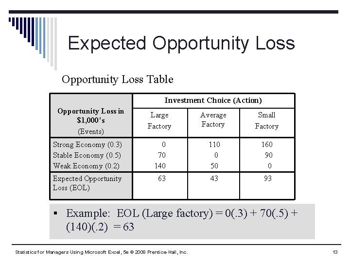
Expected Opportunity Loss Table Investment Choice (Action) Opportunity Loss in $1, 000’s (Events) Large Factory Average Factory Small Factory Strong Economy (0. 3) Stable Economy (0. 5) Weak Economy (0. 2) 0 70 140 110 0 50 160 90 0 Expected Opportunity Loss (EOL) 63 43 93 § Example: EOL (Large factory) = 0(. 3) + 70(. 5) + (140)(. 2) = 63 Statistics for Managers Using Microsoft Excel, 5 e © 2008 Prentice-Hall, Inc. 13

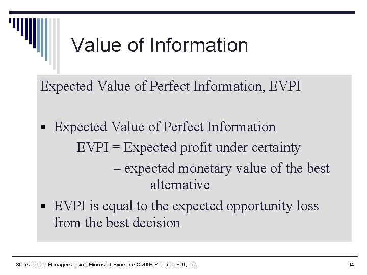
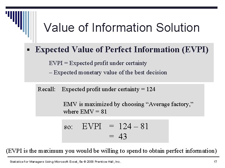
Value of Information Expected Value of Perfect Information, EVPI § Expected Value of Perfect Information EVPI = Expected profit under certainty – expected monetary value of the best alternative § EVPI is equal to the expected opportunity loss from the best decision Statistics for Managers Using Microsoft Excel, 5 e © 2008 Prentice-Hall, Inc. 14

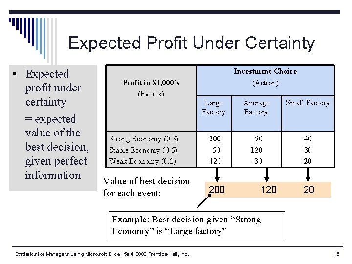
Expected Profit Under Certainty § Expected profit under certainty = expected value of the best decision, given perfect information Investment Choice (Action) Profit in $1, 000’s (Events) Strong Economy (0. 3) Stable Economy (0. 5) Weak Economy (0. 2) Value of best decision for each event: Large Factory Average Factory Small Factory 200 50 -120 90 120 -30 40 30 20 200 120 20 Example: Best decision given “Strong Economy” is “Large factory” Statistics for Managers Using Microsoft Excel, 5 e © 2008 Prentice-Hall, Inc. 15

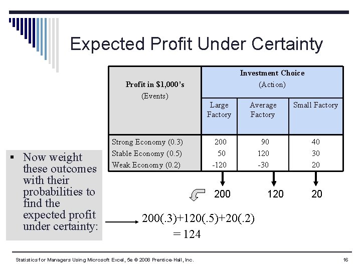
Expected Profit Under Certainty Investment Choice (Action) Profit in $1, 000’s (Events) § Now weight these outcomes with their probabilities to find the expected profit under certainty: Strong Economy (0. 3) Stable Economy (0. 5) Weak Economy (0. 2) Large Factory Average Factory Small Factory 200 50 -120 90 120 -30 40 30 20 200 120 20 200(. 3)+120(. 5)+20(. 2) = 124 Statistics for Managers Using Microsoft Excel, 5 e © 2008 Prentice-Hall, Inc. 16

Value of Information Solution § Expected Value of Perfect Information (EVPI) EVPI = Expected profit under certainty – Expected monetary value of the best decision Recall: Expected profit under certainty = 124 EMV is maximized by choosing “Average factory, ” where EMV = 81 so: EVPI = 124 – 81 = 43 (EVPI is the maximum you would be willing to spend to obtain perfect information) Statistics for Managers Using Microsoft Excel, 5 e © 2008 Prentice-Hall, Inc. 17

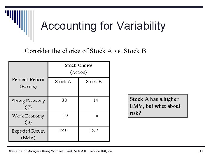
Accounting for Variability Consider the choice of Stock A vs. Stock B Stock Choice (Action) Percent Return (Events) Stock A Strong Economy (. 7) 30 14 Weak Economy (. 3) -10 8 Expected Return (EMV) 18. 0 12. 2 Stock B Statistics for Managers Using Microsoft Excel, 5 e © 2008 Prentice-Hall, Inc. Stock A has a higher EMV, but what about risk? 18

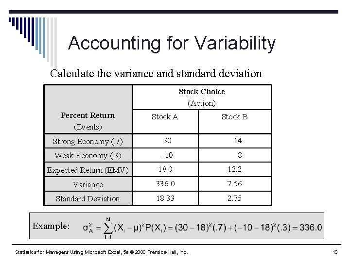
Accounting for Variability Calculate the variance and standard deviation Stock Choice (Action) Percent Return (Events) Stock A Strong Economy (. 7) 30 14 Weak Economy (. 3) -10 8 Expected Return (EMV) 18. 0 12. 2 Variance 336. 0 7. 56 Standard Deviation 18. 33 2. 75 Stock B Example: Statistics for Managers Using Microsoft Excel, 5 e © 2008 Prentice-Hall, Inc. 19

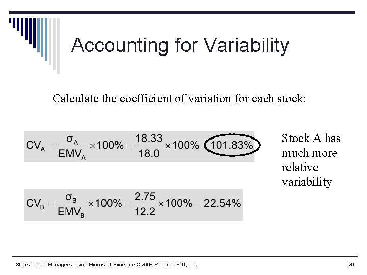
Accounting for Variability Calculate the coefficient of variation for each stock: Stock A has much more relative variability Statistics for Managers Using Microsoft Excel, 5 e © 2008 Prentice-Hall, Inc. 20

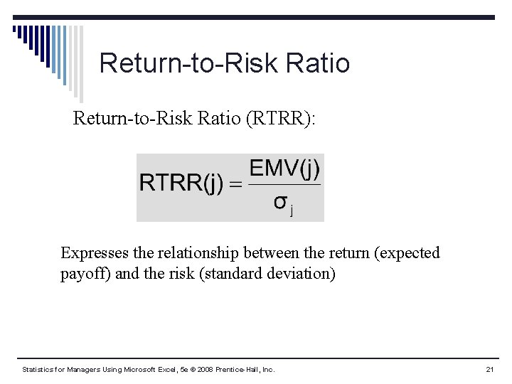
Return-to-Risk Ratio (RTRR): Expresses the relationship between the return (expected payoff) and the risk (standard deviation) Statistics for Managers Using Microsoft Excel, 5 e © 2008 Prentice-Hall, Inc. 21

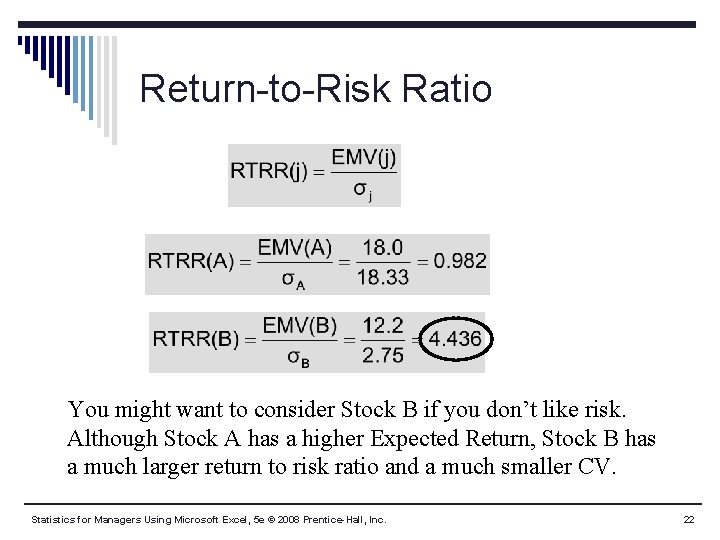
Return-to-Risk Ratio You might want to consider Stock B if you don’t like risk. Although Stock A has a higher Expected Return, Stock B has a much larger return to risk ratio and a much smaller CV. Statistics for Managers Using Microsoft Excel, 5 e © 2008 Prentice-Hall, Inc. 22

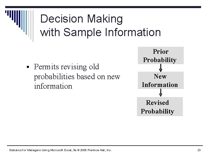
Decision Making with Sample Information § Permits revising old probabilities based on new information Prior Probability New Information Revised Probability Statistics for Managers Using Microsoft Excel, 5 e © 2008 Prentice-Hall, Inc. 23

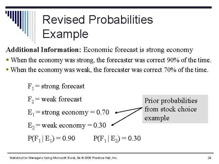
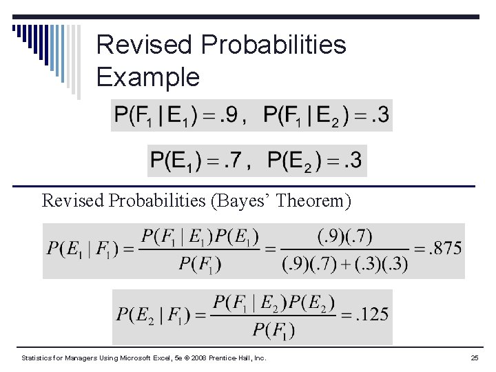
Revised Probabilities Example Additional Information: Economic forecast is strong economy § When the economy was strong, the forecaster was correct 90% of the time. § When the economy was weak, the forecaster was correct 70% of the time. F 1 = strong forecast F 2 = weak forecast E 1 = strong economy = 0. 70 E 2 = weak economy = 0. 30 P(F 1 | E 1) = 0. 90 Prior probabilities from stock choice example P(F 1 | E 2) = 0. 30 Statistics for Managers Using Microsoft Excel, 5 e © 2008 Prentice-Hall, Inc. 24

Revised Probabilities Example Revised Probabilities (Bayes’ Theorem) Statistics for Managers Using Microsoft Excel, 5 e © 2008 Prentice-Hall, Inc. 25

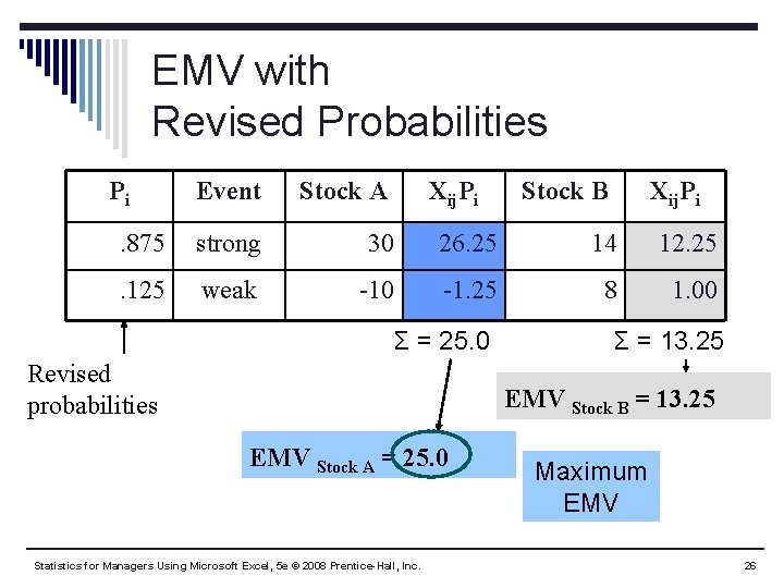
EMV with Revised Probabilities Pi Event Stock A Xij. Pi . 875 strong 30 26. 25 14 12. 25 . 125 weak -10 -1. 25 8 1. 00 Σ = 25. 0 Revised probabilities Stock B Xij. Pi Σ = 13. 25 EMV Stock B = 13. 25 EMV Stock A = 25. 0 Statistics for Managers Using Microsoft Excel, 5 e © 2008 Prentice-Hall, Inc. Maximum EMV 26

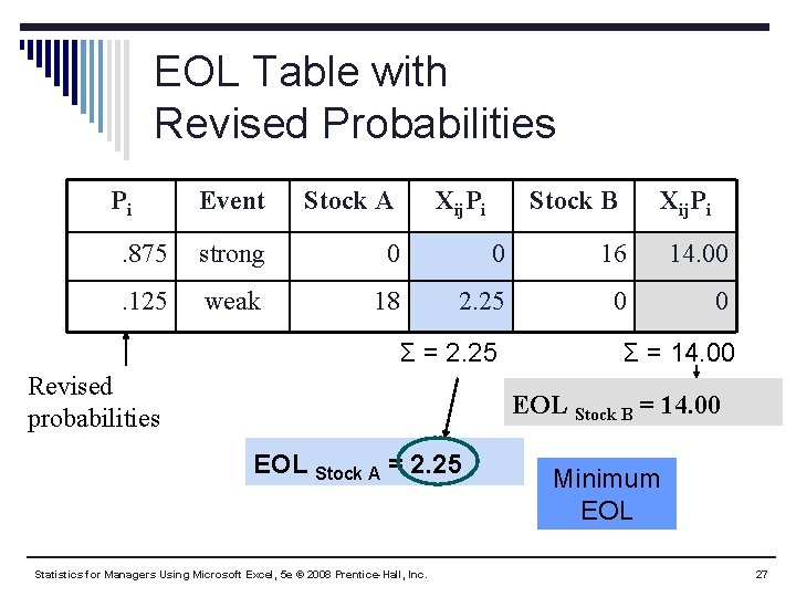
EOL Table with Revised Probabilities Pi Event Stock A Xij. Pi Stock B . 875 strong 0 0 16 14. 00 . 125 weak 18 2. 25 0 0 Σ = 2. 25 Revised probabilities Xij. Pi Σ = 14. 00 EOL Stock B = 14. 00 EOL Stock A = 2. 25 Statistics for Managers Using Microsoft Excel, 5 e © 2008 Prentice-Hall, Inc. Minimum EOL 27

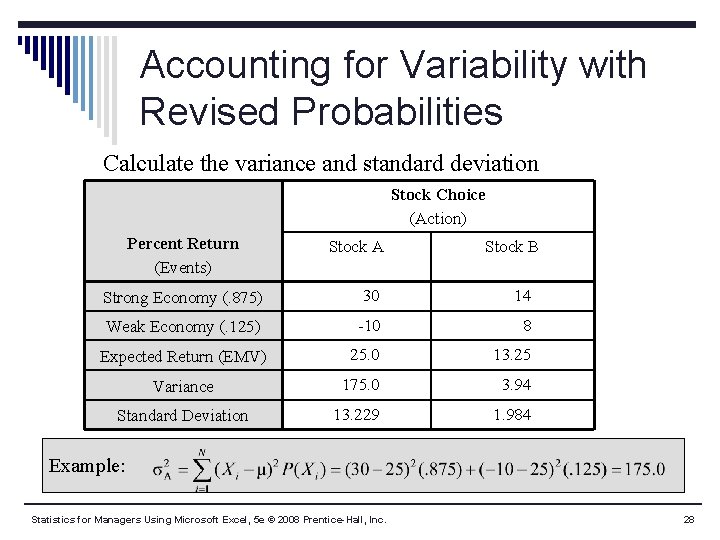
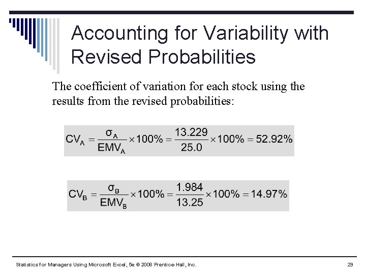
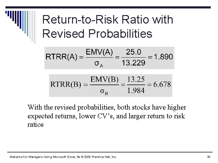
Accounting for Variability with Revised Probabilities Calculate the variance and standard deviation Stock Choice (Action) Percent Return (Events) Stock A Stock B Strong Economy (. 875) 30 14 Weak Economy (. 125) -10 8 Expected Return (EMV) 25. 0 13. 25 Variance 175. 0 3. 94 Standard Deviation 13. 229 1. 984 Example: Statistics for Managers Using Microsoft Excel, 5 e © 2008 Prentice-Hall, Inc. 28

Accounting for Variability with Revised Probabilities The coefficient of variation for each stock using the results from the revised probabilities: Statistics for Managers Using Microsoft Excel, 5 e © 2008 Prentice-Hall, Inc. 29

Return-to-Risk Ratio with Revised Probabilities With the revised probabilities, both stocks have higher expected returns, lower CV’s, and larger return to risk ratios Statistics for Managers Using Microsoft Excel, 5 e © 2008 Prentice-Hall, Inc. 30

Utility § Utility is the pleasure or satisfaction obtained from an action. § The utility of an outcome may not be the same for each individual. Statistics for Managers Using Microsoft Excel, 5 e © 2008 Prentice-Hall, Inc. 31

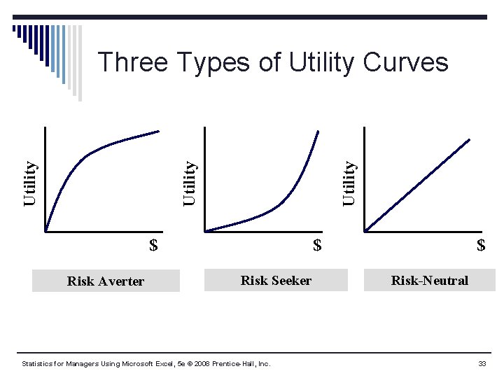
Utility Example Each incremental $1 of profit does not have the same value to every individual: §A risk averse person, once reaching a goal, assigns less utility to each incremental $1. §A risk seeker assigns more utility to each incremental $1. §A risk neutral person assigns the same utility to each extra $1. Statistics for Managers Using Microsoft Excel, 5 e © 2008 Prentice-Hall, Inc. 32

Utility Three Types of Utility Curves $ Risk Averter $ Risk Seeker Statistics for Managers Using Microsoft Excel, 5 e © 2008 Prentice-Hall, Inc. $ Risk-Neutral 33

Maximizing Expected Utility § Making decisions in terms of utility, not $ § Translate $ outcomes into utility outcomes § Calculate expected utilities for each action § Choose the action to maximize expected utility Statistics for Managers Using Microsoft Excel, 5 e © 2008 Prentice-Hall, Inc. 34

Chapter Summary In this chapter, we have § Described the payoff table and decision trees § Opportunity loss § Provided criteria for decision making § Expected monetary value § Expected opportunity loss § Return to risk ratio § Introduced expected profit under certainty and the value of perfect information § Discussed decision making with sample information § Addressed the concept of utility Statistics for Managers Using Microsoft Excel, 5 e © 2008 Prentice-Hall, Inc. 35