
Statistics for Managers Using Microsoft Excel 3 rd
- Slides: 33
Statistics for Managers Using Microsoft Excel 3 rd Edition Chapter 14 Decision Making © 2002 Prentice-Hall, Inc. Chap 14 -1
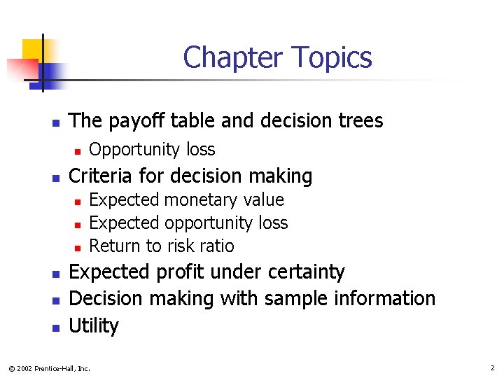
Chapter Topics n The payoff table and decision trees n n Criteria for decision making n n n Opportunity loss Expected monetary value Expected opportunity loss Return to risk ratio Expected profit under certainty Decision making with sample information Utility © 2002 Prentice-Hall, Inc. 2
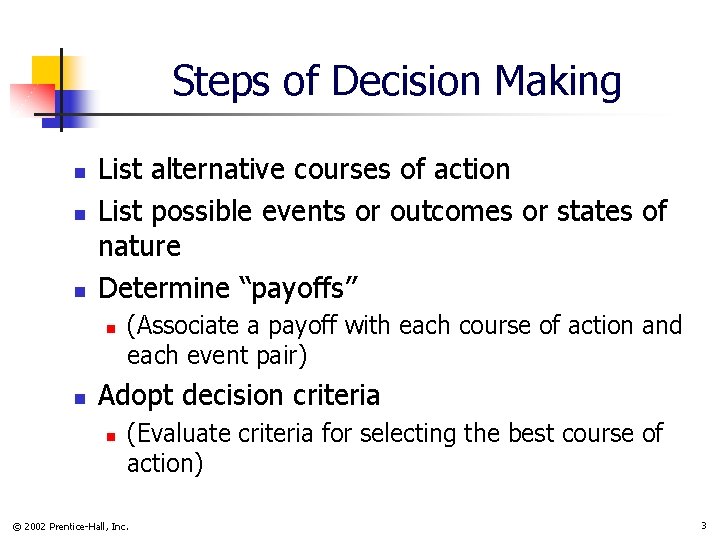
Steps of Decision Making n n n List alternative courses of action List possible events or outcomes or states of nature Determine “payoffs” n n (Associate a payoff with each course of action and each event pair) Adopt decision criteria n (Evaluate criteria for selecting the best course of action) © 2002 Prentice-Hall, Inc. 3
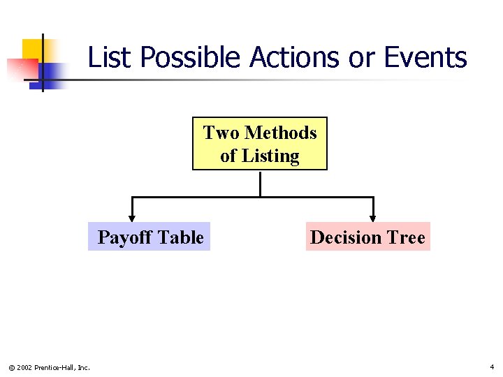
List Possible Actions or Events Two Methods of Listing Payoff Table © 2002 Prentice-Hall, Inc. Decision Tree 4
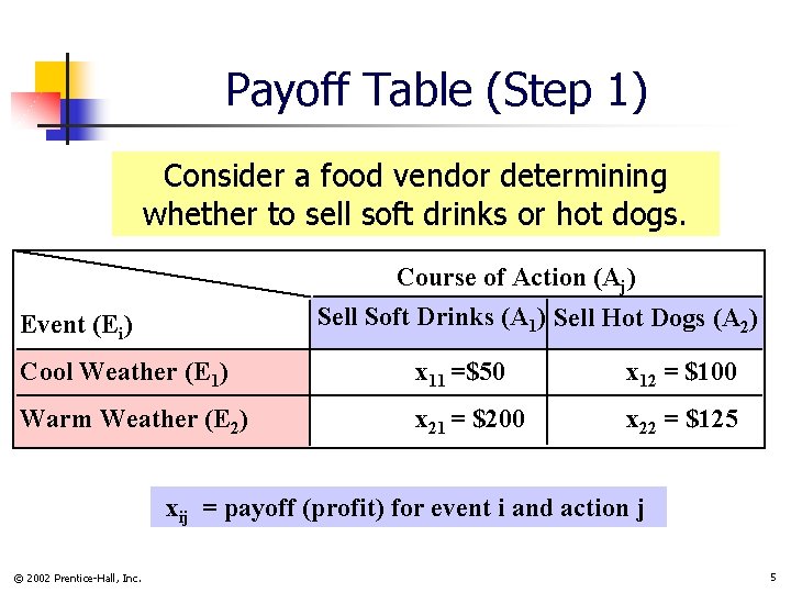
Payoff Table (Step 1) Consider a food vendor determining whether to sell soft drinks or hot dogs. Course of Action (Aj) Sell Soft Drinks (A 1) Sell Hot Dogs (A 2) Event (Ei) Cool Weather (E 1) x 11 =$50 x 12 = $100 Warm Weather (E 2) x 21 = $200 x 22 = $125 xij = payoff (profit) for event i and action j © 2002 Prentice-Hall, Inc. 5
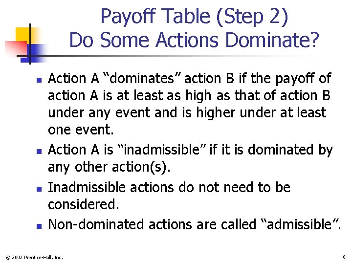
Payoff Table (Step 2) Do Some Actions Dominate? n n Action A “dominates” action B if the payoff of action A is at least as high as that of action B under any event and is higher under at least one event. Action A is “inadmissible” if it is dominated by any other action(s). Inadmissible actions do not need to be considered. Non-dominated actions are called “admissible”. © 2002 Prentice-Hall, Inc. 6
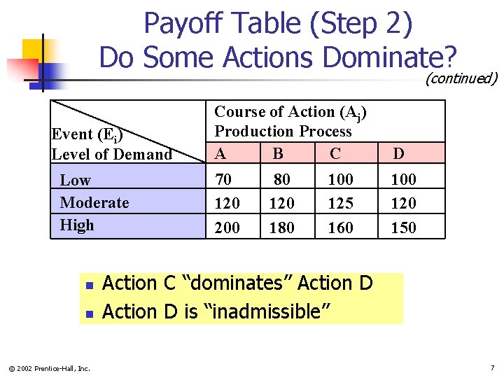
Payoff Table (Step 2) Do Some Actions Dominate? (continued) Event (Ei) Level of Demand Low Moderate High n n © 2002 Prentice-Hall, Inc. Course of Action (Aj) Production Process A B C D 70 120 200 120 150 80 120 180 100 125 160 Action C “dominates” Action D is “inadmissible” 7
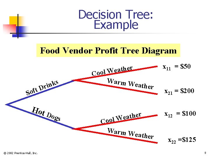
Decision Tree: Example Food Vendor Profit Tree Diagram Soft s k n i Dr Hot Dog s x 11 = $50 her t a e W l Coo Warm W eather er h t a e ool W C Warm W eather © 2002 Prentice-Hall, Inc. x 21 = $200 x 12 = $100 x 22 =$125 8
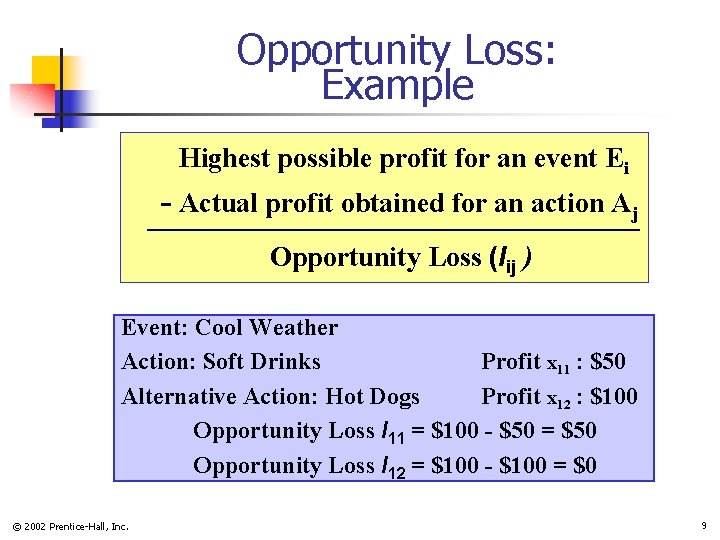
Opportunity Loss: Example Highest possible profit for an event Ei - Actual profit obtained for an action Aj Opportunity Loss (lij ) Event: Cool Weather Action: Soft Drinks Profit x 11 : $50 Alternative Action: Hot Dogs Profit x 12 : $100 Opportunity Loss l 11 = $100 - $50 = $50 Opportunity Loss l 12 = $100 - $100 = $0 © 2002 Prentice-Hall, Inc. 9
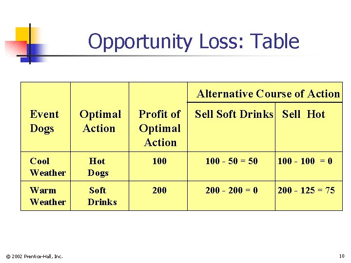
Opportunity Loss: Table Alternative Course of Action Event Dogs Optimal Action Profit of Optimal Action Cool Weather Hot Dogs 100 - 50 = 50 100 - 100 = 0 Warm Weather Soft Drinks 200 - 200 = 0 200 - 125 = 75 © 2002 Prentice-Hall, Inc. Sell Soft Drinks Sell Hot 10
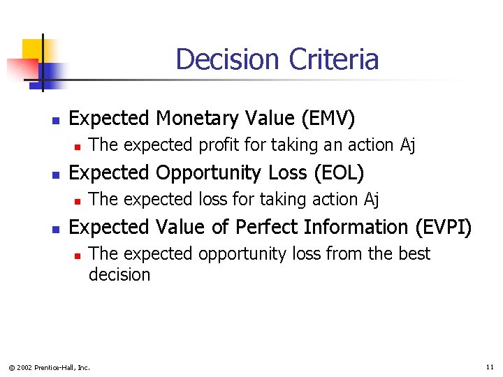
Decision Criteria n Expected Monetary Value (EMV) n n Expected Opportunity Loss (EOL) n n The expected profit for taking an action Aj The expected loss for taking action Aj Expected Value of Perfect Information (EVPI) n The expected opportunity loss from the best decision © 2002 Prentice-Hall, Inc. 11
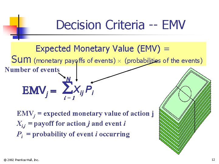
Decision Criteria -- EMV Expected Monetary Value (EMV) = Sum (monetary payoffs of events) (probabilities of the events) Number of events N Vj Xij Pi i=1 EMVj = expected monetary value of action j Xi, j = payoff for action j and event i Pi = probability of event i occurring © 2002 Prentice-Hall, Inc. 12
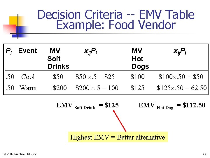
Decision Criteria -- EMV Table Example: Food Vendor Pi Event. 50 Cool . 50 Warm MV xij. Pi Soft Drinks $50 . 5 = $25 $200 . 5 = 100 EMV Soft Drink = $125 MV Hot Dogs $100 xij. Pi $100. 50 = $50 $125. 50 = 62. 50 EMV Hot Dog = $112. 50 Highest EMV = Better alternative © 2002 Prentice-Hall, Inc. 13
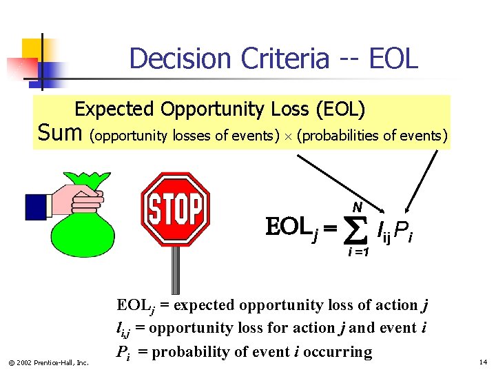
Decision Criteria -- EOL Expected Opportunity Loss (EOL) Sum (opportunity losses of events) (probabilities of events) Lj N lij Pi i =1 © 2002 Prentice-Hall, Inc. EOLj = expected opportunity loss of action j li, j = opportunity loss for action j and event i Pi = probability of event i occurring 14
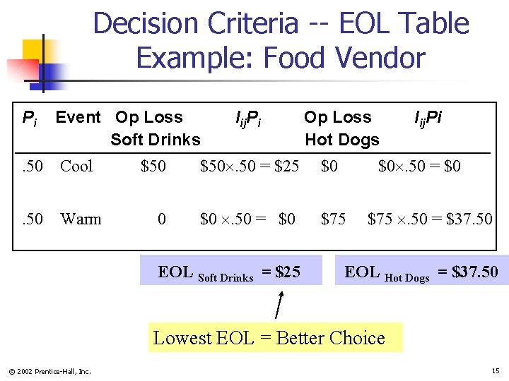
Decision Criteria -- EOL Table Example: Food Vendor Pi Event Op Loss Soft Drinks . 50 Cool . 50 Warm lij. Pi Op Loss Hot Dogs $50. 50 = $25 $0 0 $0 . 50 = $0 $75 EOL Soft Drinks = $25 lij. Pi $0. 50 = $0 $75 . 50 = $37. 50 EOL Hot Dogs = $37. 50 Lowest EOL = Better Choice © 2002 Prentice-Hall, Inc. 15
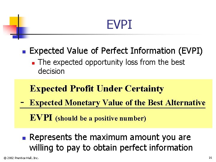
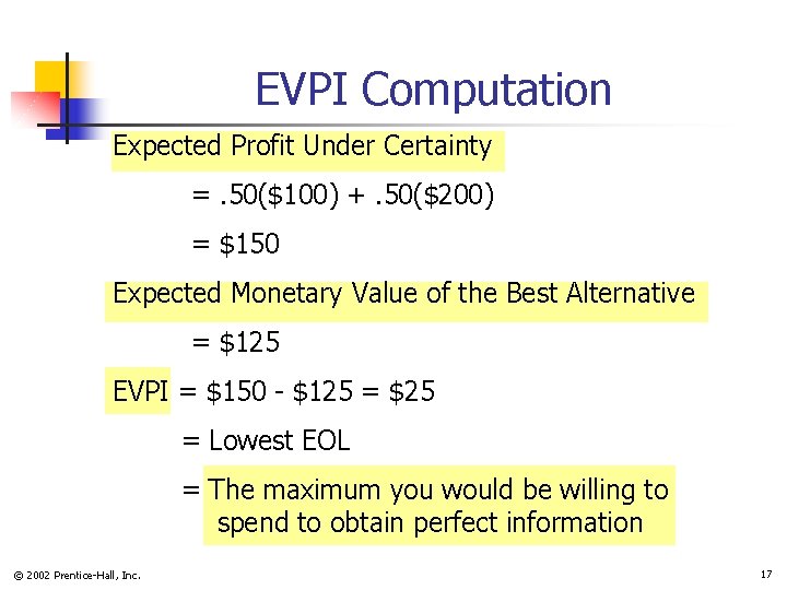
EVPI n Expected Value of Perfect Information (EVPI) n The expected opportunity loss from the best decision Expected Profit Under Certainty - Expected Monetary Value of the Best Alternative EVPI (should be a positive number) n Represents the maximum amount you are willing to pay to obtain perfect information © 2002 Prentice-Hall, Inc. 16
EVPI Computation Expected Profit Under Certainty =. 50($100) +. 50($200) = $150 Expected Monetary Value of the Best Alternative = $125 EVPI = $150 - $125 = $25 = Lowest EOL = The maximum you would be willing to spend to obtain perfect information © 2002 Prentice-Hall, Inc. 17
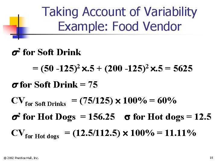
Taking Account of Variability Example: Food Vendor 2 for Soft Drink = (50 -125)2 . 5 + (200 -125)2 . 5 = 5625 for Soft Drink = 75 CVfor Soft Drinks = (75/125) 100% = 60% 2 for Hot Dogs = 156. 25 for Hot dogs = 12. 5 CVfor Hot dogs = (12. 5/112. 5) 100% = 11. 11% © 2002 Prentice-Hall, Inc. 18
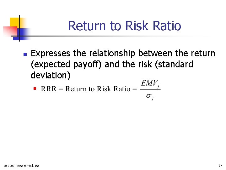
Return to Risk Ratio n Expresses the relationship between the return (expected payoff) and the risk (standard deviation) n © 2002 Prentice-Hall, Inc. 19
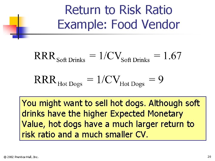
Return to Risk Ratio Example: Food Vendor You might want to sell hot dogs. Although soft drinks have the higher Expected Monetary Value, hot dogs have a much larger return to risk ratio and a much smaller CV. © 2002 Prentice-Hall, Inc. 20
Decision Making in PHStat | decision-making | expected monetary value n n Check the “expected opportunity loss” and “measures of valuation” boxes Excel spreadsheet for the food vendor example © 2002 Prentice-Hall, Inc. 21
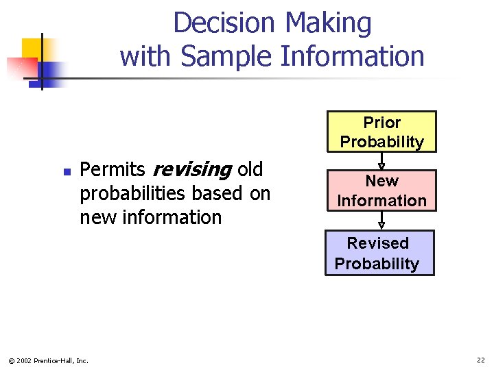
Decision Making with Sample Information Prior Probability n Permits revising old probabilities based on new information New Information Revised Probability © 2002 Prentice-Hall, Inc. 22
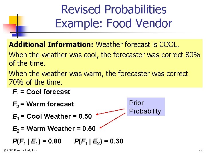
Revised Probabilities Example: Food Vendor Additional Information: Weather forecast is COOL. When the weather was cool, the forecaster was correct 80% of the time. When the weather was warm, the forecaster was correct 70% of the time. F 1 = Cool forecast F 2 = Warm forecast E 1 = Cool Weather = 0. 50 Prior Probability E 2 = Warm Weather = 0. 50 P(F 1 | E 1) = 0. 80 © 2002 Prentice-Hall, Inc. P(F 1 | E 2) = 0. 30 23
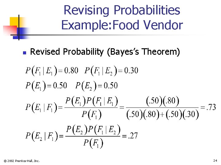
Revising Probabilities Example: Food Vendor n Revised Probability (Bayes’s Theorem) © 2002 Prentice-Hall, Inc. 24
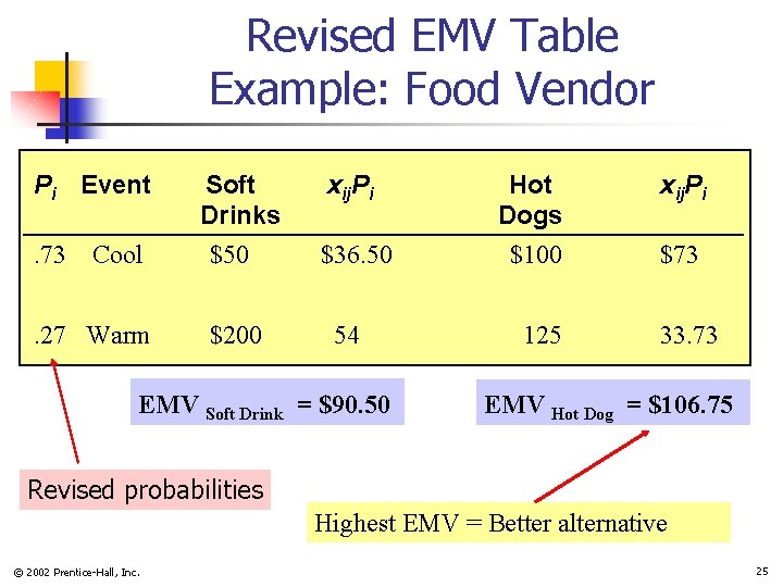
Revised EMV Table Example: Food Vendor Pi Event. 73 Cool . 27 Warm Soft Drinks $50 $200 xij. Pi $36. 50 54 EMV Soft Drink = $90. 50 Hot Dogs $100 125 xij. Pi $73 33. 73 EMV Hot Dog = $106. 75 Revised probabilities Highest EMV = Better alternative © 2002 Prentice-Hall, Inc. 25
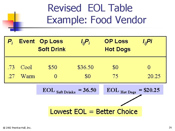
Revised EOL Table Example: Food Vendor Pi Event Op Loss Soft Drink . 73 Cool . 27 Warm $50 0 lij. Pi $36. 50 $0 EOL Soft Drinks = 36. 50 OP Loss Hot Dogs lij. Pi $0 0 75 20. 25 EOL Hot Dogs = $20. 25 Lowest EOL = Better Choice © 2002 Prentice-Hall, Inc. 26
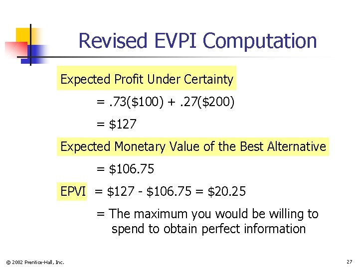
Revised EVPI Computation Expected Profit Under Certainty =. 73($100) +. 27($200) = $127 Expected Monetary Value of the Best Alternative = $106. 75 EPVI = $127 - $106. 75 = $20. 25 = The maximum you would be willing to spend to obtain perfect information © 2002 Prentice-Hall, Inc. 27
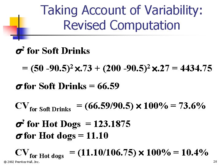
Taking Account of Variability: Revised Computation 2 for Soft Drinks = (50 -90. 5)2 . 73 + (200 -90. 5)2 . 27 = 4434. 75 for Soft Drinks = 66. 59 CVfor Soft Drinks = (66. 59/90. 5) 100% = 73. 6% 2 for Hot Dogs = 123. 1875 for Hot dogs = 11. 10 CVfor Hot dogs = (11. 10/106. 75) 100% = 10. 4% © 2002 Prentice-Hall, Inc. 28
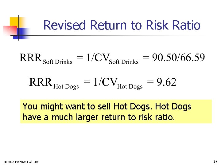
Revised Return to Risk Ratio You might want to sell Hot Dogs have a much larger return to risk ratio. © 2002 Prentice-Hall, Inc. 29
Revised Decision Making in PHStat | decision-making | expected monetary value n n n Check the “expected opportunity loss” and “measures of valuation” boxes Use the revised probabilities Excel spreadsheet for the food vendor example © 2002 Prentice-Hall, Inc. 30
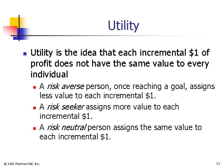
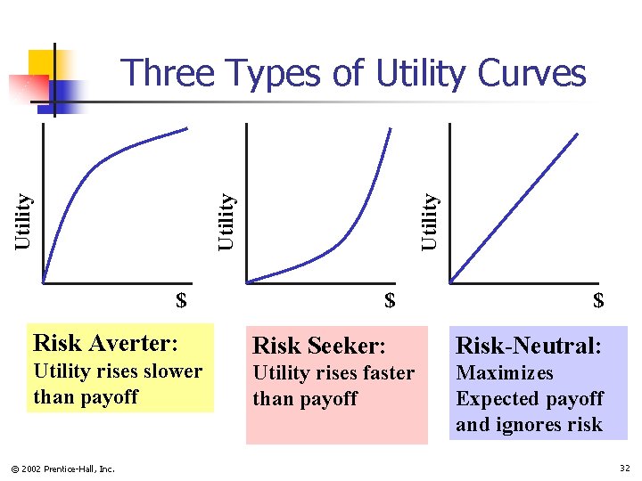
Utility n Utility is the idea that each incremental $1 of profit does not have the same value to every individual n n n A risk averse person, once reaching a goal, assigns less value to each incremental $1. A risk seeker assigns more value to each incremental $1. A risk neutral person assigns the same value to each incremental $1. © 2002 Prentice-Hall, Inc. 31
$ Risk Averter: Utility rises slower than payoff © 2002 Prentice-Hall, Inc. Utility Three Types of Utility Curves $ $ Risk Seeker: Risk-Neutral: Utility rises faster than payoff Maximizes Expected payoff and ignores risk 32
Chapter Summary n Described the payoff table and decision trees n n Provided criteria for decision making n n n Opportunity loss Expected monetary value Expected opportunity loss Return to risk ratio Introduced expected profit under certainty Discussed decision making with sample information Addressed the concept of utility © 2002 Prentice-Hall, Inc. 33