Statistics for Business and Economics Chapter 8 Design

Statistics for Business and Economics Chapter 8 Design of Experiments and Analysis of Variance

Learning Objectives 1. Describe Analysis of Variance (ANOVA) 2. Explain the Rationale of ANOVA 3. Compare Experimental Designs 4. Test the Equality of 2 or More Means • • Completely Randomized Design Factorial Design

Experiments

Experiment • Investigator controls one or more independent variables – Called treatment variables or factors – Contain two or more levels (subcategories) • Observes effect on dependent variable – Response to levels of independent variable • Experimental design: plan used to test hypotheses

Examples of Experiments 1. Thirty stores are randomly assigned 1 of 4 (levels) store displays (independent variable) to see the effect on sales (dependent variable). 2. Two hundred consumers are randomly assigned 1 of 3 (levels) brands of juice (independent variable) to study reaction (dependent variable).

Experimental Designs Completely Randomized Factorial One-Way ANOVA Two-Way ANOVA

Completely Randomized Design

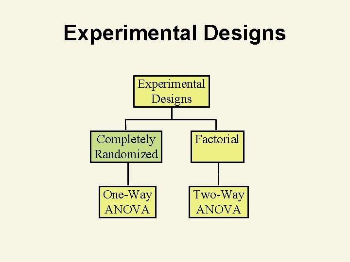
Experimental Designs Completely Randomized Factorial One-Way ANOVA Two-Way ANOVA

Completely Randomized Design • Experimental units (subjects) are assigned randomly to treatments – Subjects are assumed homogeneous • One factor or independent variable – Two or more treatment levels or classifications • Analyzed by one-way ANOVA

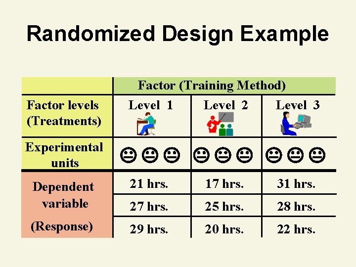
Randomized Design Example Factor (Training Method) Factor levels (Treatments) Experimental units Level 1 Level 2 Level 3 Dependent variable 21 hrs. 17 hrs. 31 hrs. 27 hrs. 25 hrs. 28 hrs. (Response) 29 hrs. 20 hrs. 22 hrs.

One-Way ANOVA F-Test

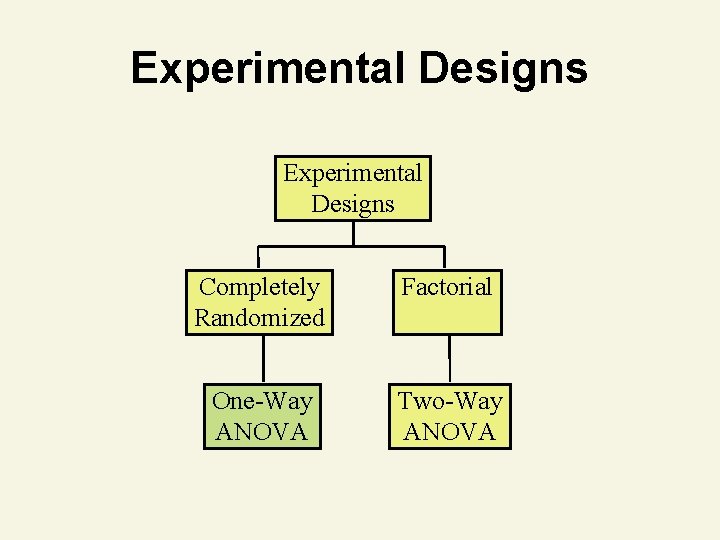
Experimental Designs Completely Randomized Factorial One-Way ANOVA Two-Way ANOVA

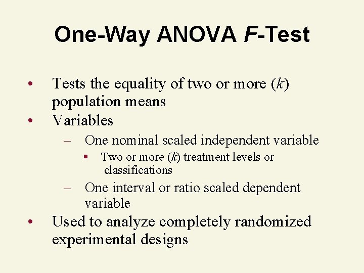
One-Way ANOVA F-Test • • Tests the equality of two or more (k) population means Variables – One nominal scaled independent variable § Two or more (k) treatment levels or classifications – One interval or ratio scaled dependent variable • Used to analyze completely randomized experimental designs

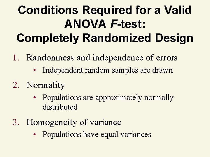
Conditions Required for a Valid ANOVA F-test: Completely Randomized Design 1. Randomness and independence of errors • Independent random samples are drawn 2. Normality • Populations are approximately normally distributed 3. Homogeneity of variance • Populations have equal variances

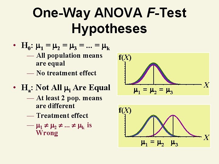
One-Way ANOVA F-Test Hypotheses • H 0: 1 = 2 = 3 =. . . = k — All population means are equal — No treatment effect f(X) • Ha: Not All i Are Equal — At least 2 pop. means are different — Treatment effect — 1 2 . . . k is Wrong 1 = 2 = 3 X f(X) 1 = 2 3 X

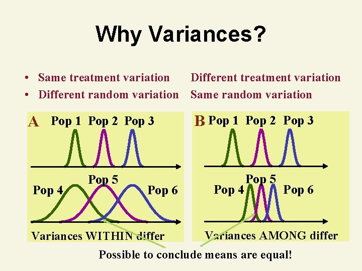
Why Variances? • Same treatment variation Different treatment variation • Different random variation Same random variation A Pop 1 Pop 2 Pop 3 Pop 4 Pop 5 Pop 6 Variances WITHIN differ B Pop 1 Pop 4 Pop 2 Pop 3 Pop 5 Pop 6 Variances AMONG differ Possible to conclude means are equal!

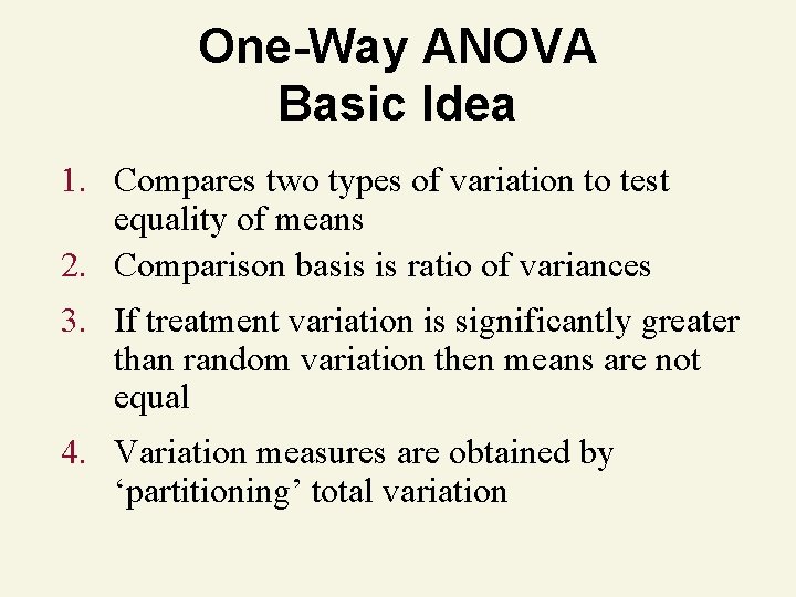
One-Way ANOVA Basic Idea 1. Compares two types of variation to test equality of means 2. Comparison basis is ratio of variances 3. If treatment variation is significantly greater than random variation then means are not equal 4. Variation measures are obtained by ‘partitioning’ total variation

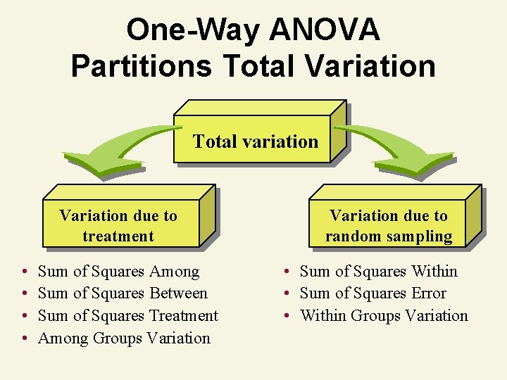
One-Way ANOVA Partitions Total Variation Total variation Variation due to treatment • • Sum of Squares Among Sum of Squares Between Sum of Squares Treatment Among Groups Variation due to random sampling • Sum of Squares Within • Sum of Squares Error • Within Groups Variation

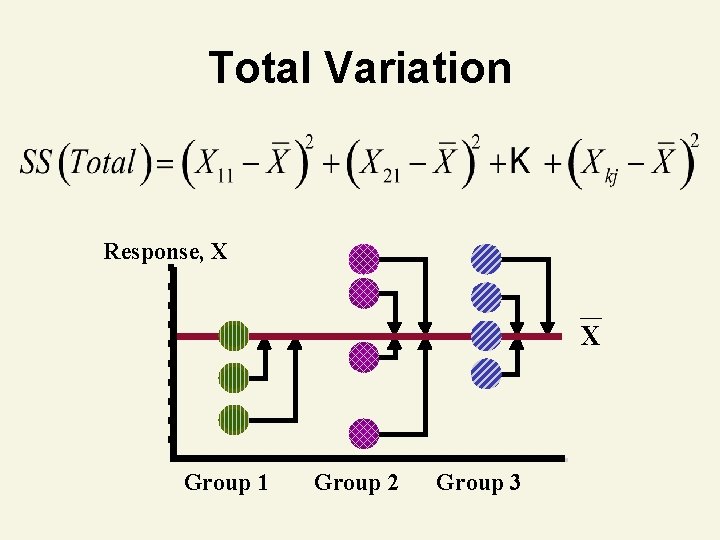
Total Variation Response, X X Group 1 Group 2 Group 3

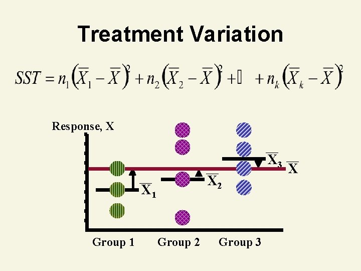
Treatment Variation Response, X X 3 X 2 X 1 Group 2 Group 3 X

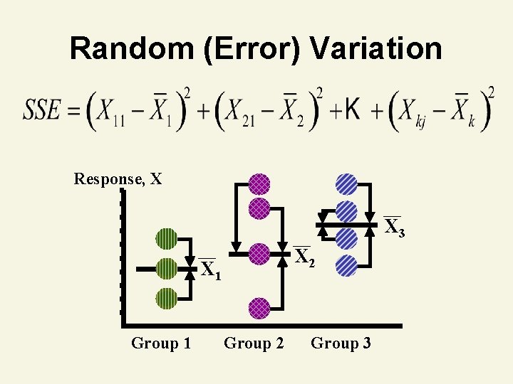
Random (Error) Variation Response, X X 3 X 2 X 1 Group 2 Group 3

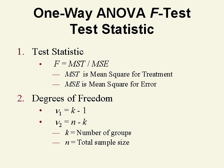
One-Way ANOVA F-Test Statistic 1. Test Statistic • F = MST / MSE — MST is Mean Square for Treatment — MSE is Mean Square for Error 2. Degrees of Freedom • • 1 = k - 1 2 = n - k — k = Number of groups — n = Total sample size

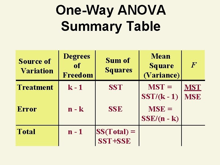
One-Way ANOVA Summary Table Source of Variation Degrees of Freedom Sum of Squares Treatment k-1 SST Error n-k SSE Total n-1 SS(Total) = SST+SSE Mean F Square (Variance) MST = MST SST/(k - 1) MSE = SSE/(n - k)

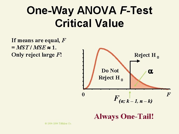
One-Way ANOVA F-Test Critical Value If means are equal, F = MST / MSE 1. Only reject large F! Reject H 0 Do Not Reject H 0 0 F(α; k – 1, n – k) Always One-Tail! © 1984 -1994 T/Maker Co. F

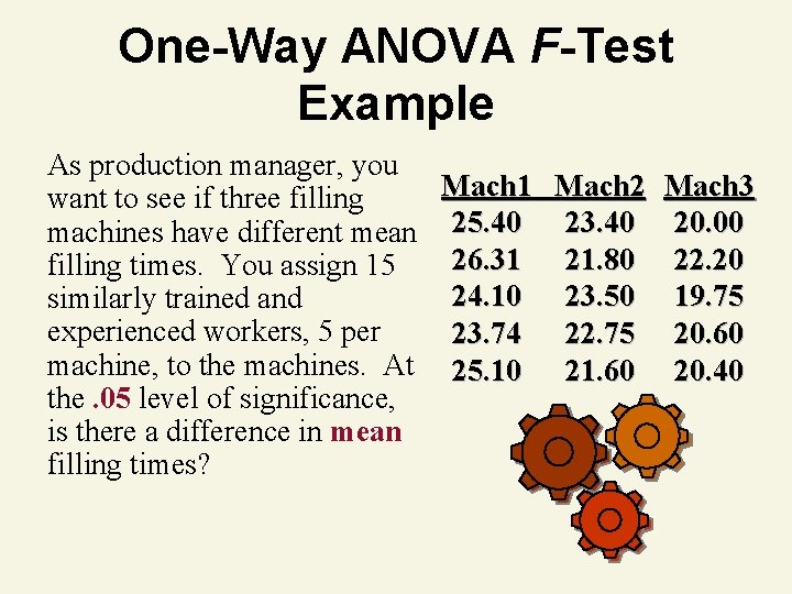
One-Way ANOVA F-Test Example As production manager, you Mach 1 Mach 2 Mach 3 want to see if three filling machines have different mean 25. 40 23. 40 20. 00 26. 31 21. 80 22. 20 filling times. You assign 15 24. 10 23. 50 19. 75 similarly trained and experienced workers, 5 per 23. 74 22. 75 20. 60 machine, to the machines. At 25. 10 21. 60 20. 40 the. 05 level of significance, is there a difference in mean filling times?

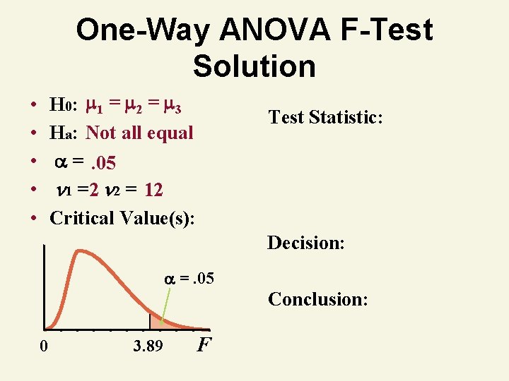
One-Way ANOVA F-Test Solution H 0: 1 = 2 = 3 Ha: Not all equal =. 05 1 = 2 2 = 12 Critical Value(s): • • • Test Statistic: Decision: =. 05 Conclusion: 0 3. 89 F

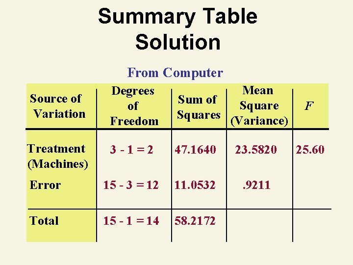
Summary Table Solution From Computer Source of Variation Degrees of Freedom Mean Sum of Squares (Variance) Treatment (Machines) 3 -1=2 47. 1640 23. 5820 Error 15 - 3 = 12 11. 0532 . 9211 Total 15 - 1 = 14 58. 2172 F 25. 60

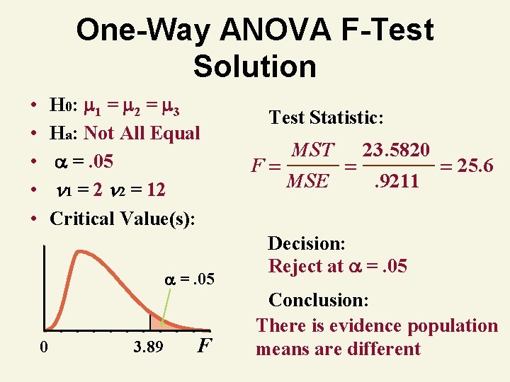
One-Way ANOVA F-Test Solution H 0: 1 = 2 = 3 Ha: Not All Equal =. 05 1 = 2 2 = 12 Critical Value(s): • • • =. 05 0 3. 89 F Test Statistic: F MST MSE 23. 5820. 9211 25. 6 Decision: Reject at =. 05 Conclusion: There is evidence population means are different

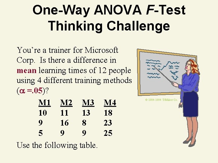
One-Way ANOVA F-Test Thinking Challenge You’re a trainer for Microsoft Corp. Is there a difference in mean learning times of 12 people using 4 different training methods ( =. 05)? M 1 M 2 M 3 M 4 10 11 13 18 9 16 8 23 5 9 9 25 Use the following table. © 1984 -1994 T/Maker Co.

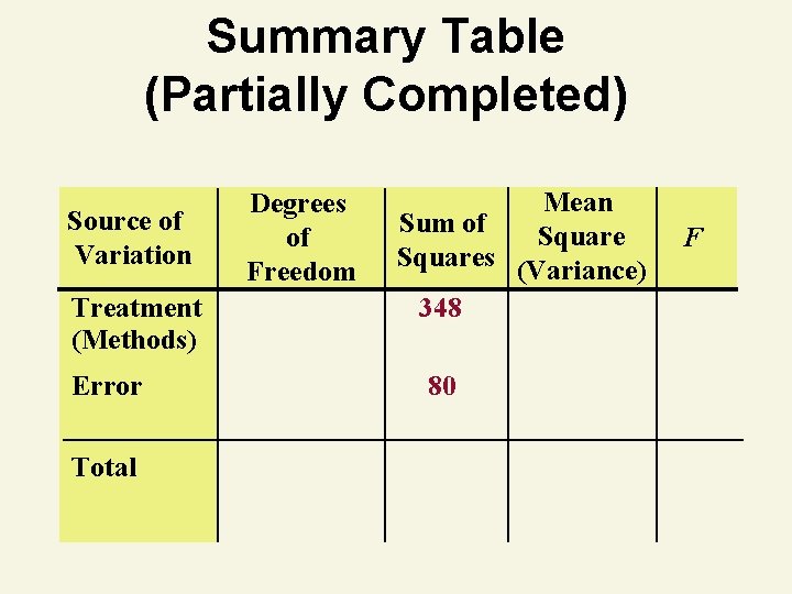
Summary Table (Partially Completed) Source of Variation Treatment (Methods) Error Total Degrees of Freedom Mean Sum of Squares (Variance) 348 80 F

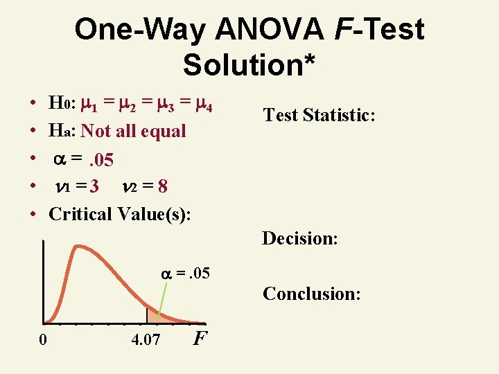
One-Way ANOVA F-Test Solution* H 0: 1 = 2 = 3 = 4 Ha: Not all equal =. 05 1 = 3 2 = 8 Critical Value(s): • • • Test Statistic: Decision: =. 05 Conclusion: 0 4. 07 F

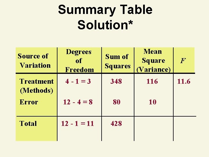
Summary Table Solution* Source of Variation Degrees of Freedom Mean Sum of Squares (Variance) Treatment (Methods) 4 -1=3 348 116 Error 12 - 4 = 8 80 10 Total 12 - 1 = 11 428 F 11. 6

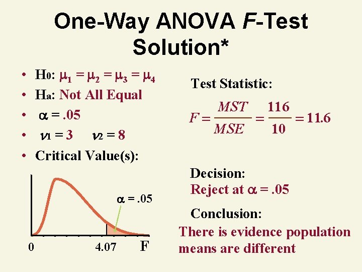
One-Way ANOVA F-Test Solution* H 0: 1 = 2 = 3 = 4 Ha: Not All Equal =. 05 1 = 3 2 = 8 Critical Value(s): • • • =. 05 0 4. 07 F Test Statistic: F MST MSE 116 10 11. 6 Decision: Reject at =. 05 Conclusion: There is evidence population means are different

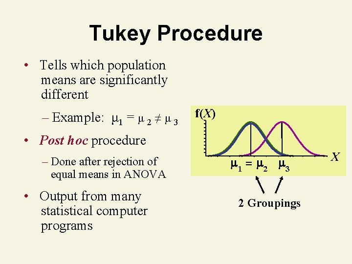
Tukey Procedure • Tells which population means are significantly different – Example: μ 1 = μ 2 ≠ μ 3 f(X) • Post hoc procedure – Done after rejection of equal means in ANOVA • Output from many statistical computer programs 1 = 2 3 2 Groupings X

Randomized Block Design • • • Reduces sampling variability (MSE) Matched sets of experimental units (blocks) One experimental unit from each block is randomly assigned to each treatment

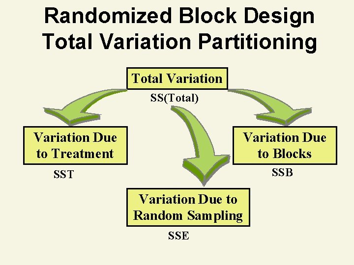
Randomized Block Design Total Variation Partitioning Total Variation SS(Total) Variation Due to Treatment Variation Due to Blocks SSB SST Variation Due to Random Sampling SSE

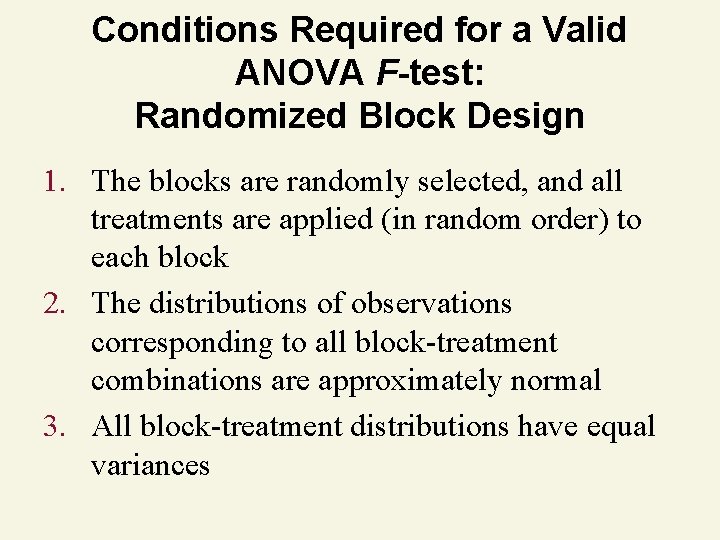
Conditions Required for a Valid ANOVA F-test: Randomized Block Design 1. The blocks are randomly selected, and all treatments are applied (in random order) to each block 2. The distributions of observations corresponding to all block-treatment combinations are approximately normal 3. All block-treatment distributions have equal variances

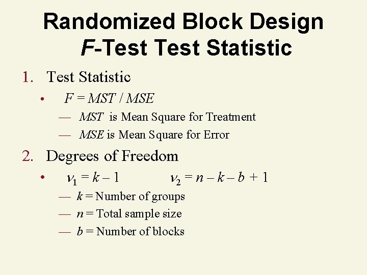
Randomized Block Design F-Test Statistic 1. Test Statistic • F = MST / MSE — MST is Mean Square for Treatment — MSE is Mean Square for Error 2. Degrees of Freedom • 1 = k – 1 2 = n – k – b + 1 — k = Number of groups — n = Total sample size — b = Number of blocks

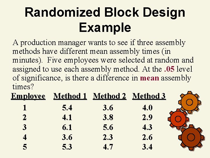
Randomized Block Design Example A production manager wants to see if three assembly methods have different mean assembly times (in minutes). Five employees were selected at random and assigned to use each assembly method. At the. 05 level of significance, is there a difference in mean assembly times? Employee Method 1 Method 2 Method 3 1 5. 4 3. 6 4. 0 2 4. 1 3. 8 2. 9 3 6. 1 5. 6 4. 3 4 3. 6 2. 3 2. 6 5 5. 3 4. 7 3. 4

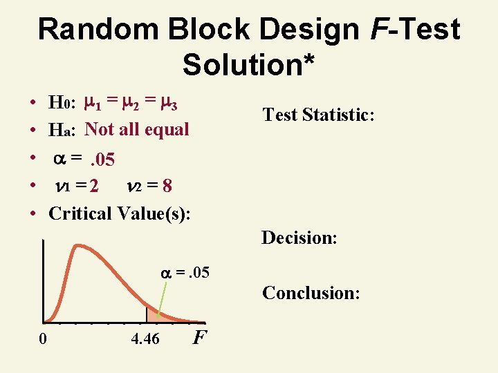
Random Block Design F-Test Solution* H 0: 1 = 2 = 3 Ha: Not all equal =. 05 1 = 2 2 = 8 Critical Value(s): • • • Test Statistic: Decision: =. 05 Conclusion: 0 4. 46 F

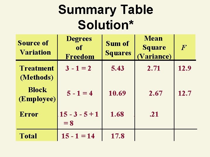
Summary Table Solution* Source of Variation Degrees of Freedom Mean Sum of Squares (Variance) F Treatment (Methods) 3 -1=2 5. 43 2. 71 12. 9 Block (Employee) 5 -1=4 10. 69 2. 67 12. 7 Error 15 - 3 - 5 + 1 =8 1. 68 . 21 Total 15 - 1 = 14 17. 8

Random Block Design F-Test Solution* H 0: 1 = 2 = 3 Ha: Not all equal =. 05 1 = 2 2 = 8 Critical Value(s): • • • Test Statistic: F =. 05 0 4. 46 F MST MSE 2. 71. 21 12. 9 Decision: Reject at =. 05 Conclusion: There is evidence population means are different

Factorial Experiments

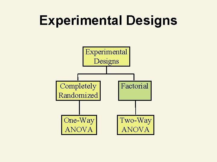
Experimental Designs Completely Randomized Factorial One-Way ANOVA Two-Way ANOVA

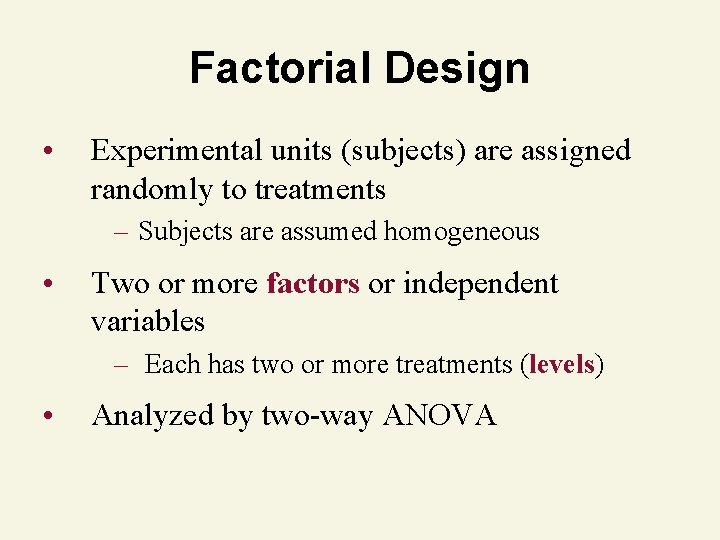
Factorial Design • Experimental units (subjects) are assigned randomly to treatments – Subjects are assumed homogeneous • Two or more factors or independent variables – Each has two or more treatments (levels) • Analyzed by two-way ANOVA

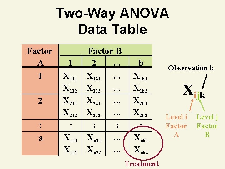
Two-Way ANOVA Data Table Factor A 1 2 : a 1 X 112 X 211 X 212 : Xa 11 Xa 12 Factor B 2. . . X 121. . . X 122. . . X 221. . . X 222. . . : : Xa 21. . . Xa 22. . . b X 1 b 1 X 1 b 2 X 2 b 1 X 2 b 2 : Xab 1 Xab 2 Treatment Observation k Xijk Level i Factor A Level j Factor B

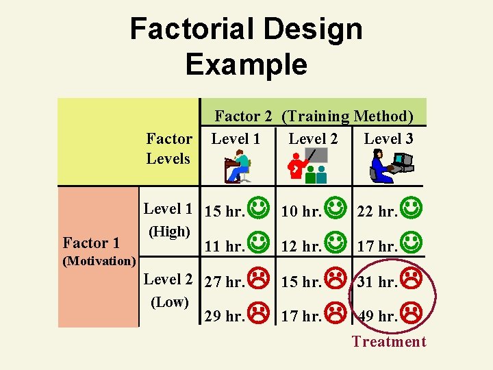
Factorial Design Example Factor Levels Factor 2 (Training Method) Level 1 Level 2 Level 3 11 hr. 27 hr. 29 hr. Level 1 15 hr. Factor 1 (High) (Motivation) Level 2 (Low) 12 hr. 15 hr. 17 hr. 10 hr. 17 hr. 31 hr. 49 hr. 22 hr. Treatment

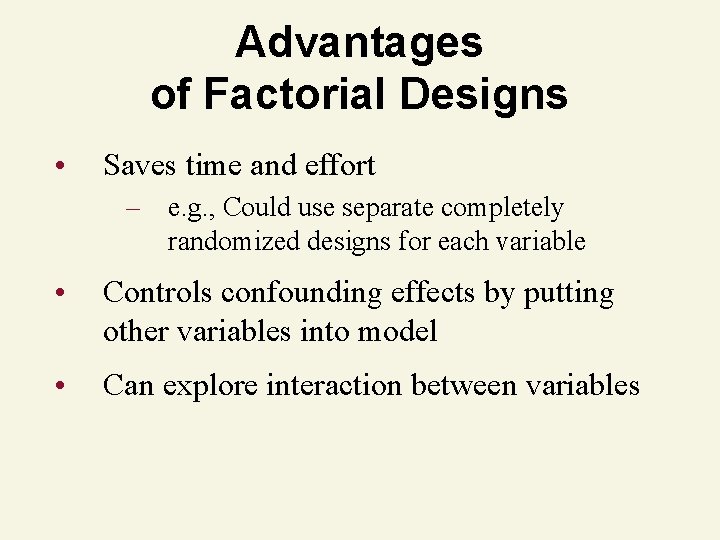
Advantages of Factorial Designs • Saves time and effort – e. g. , Could use separate completely randomized designs for each variable • Controls confounding effects by putting other variables into model • Can explore interaction between variables

Two-Way ANOVA

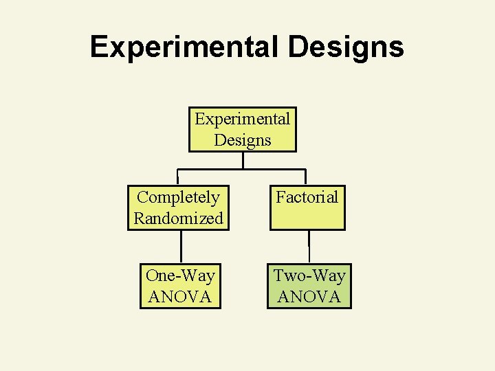
Experimental Designs Completely Randomized Factorial One-Way ANOVA Two-Way ANOVA

Two-Way ANOVA • Tests the equality of two or more population means when several independent variables are used • Same results as separate one-way ANOVA on each variable – No interaction can be tested • Used to analyze factorial designs

Interaction • Occurs when effects of one factor vary according to levels of other factor • When significant, interpretation of main effects (A and B) is complicated • Can be detected – In data table, pattern of cell means in one row differs from another row – In graph of cell means, lines cross

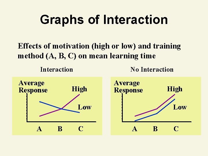
Graphs of Interaction Effects of motivation (high or low) and training method (A, B, C) on mean learning time Interaction Average Response No Interaction High Average Response High Low A B C

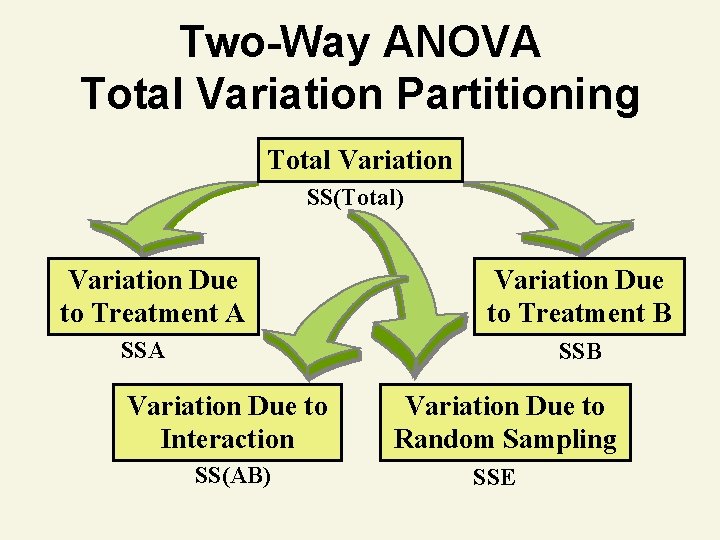
Two-Way ANOVA Total Variation Partitioning Total Variation SS(Total) Variation Due to Treatment A Variation Due to Treatment B SSA SSB Variation Due to Interaction SS(AB) Variation Due to Random Sampling SSE

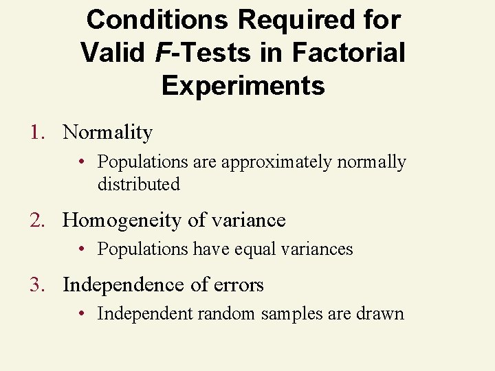
Conditions Required for Valid F-Tests in Factorial Experiments 1. Normality • Populations are approximately normally distributed 2. Homogeneity of variance • Populations have equal variances 3. Independence of errors • Independent random samples are drawn

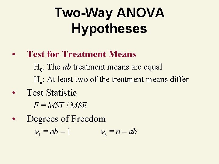
Two-Way ANOVA Hypotheses • Test for Treatment Means H 0: The ab treatment means are equal Ha: At least two of the treatment means differ • Test Statistic F = MST / MSE • Degrees of Freedom 1 = ab – 1 2 = n – ab

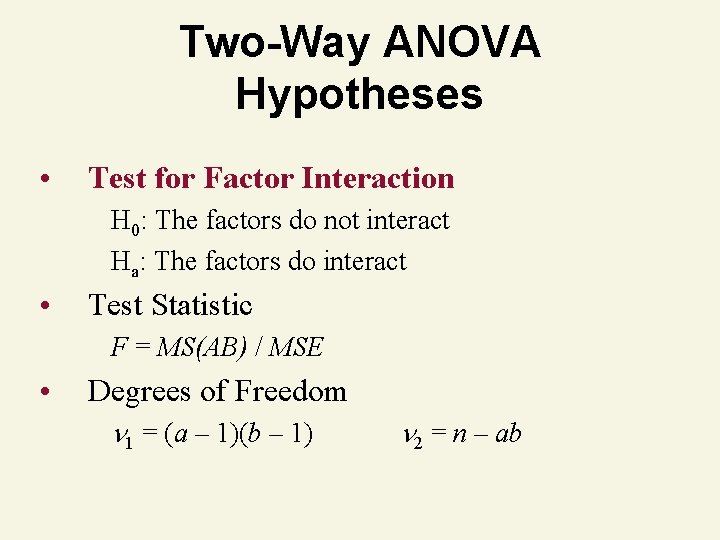
Two-Way ANOVA Hypotheses • Test for Factor Interaction H 0: The factors do not interact Ha: The factors do interact • Test Statistic F = MS(AB) / MSE • Degrees of Freedom 1 = (a – 1)(b – 1) 2 = n – ab

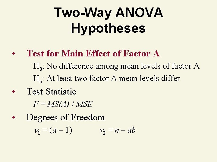
Two-Way ANOVA Hypotheses • Test for Main Effect of Factor A H 0: No difference among mean levels of factor A Ha: At least two factor A mean levels differ • Test Statistic F = MS(A) / MSE • Degrees of Freedom 1 = (a – 1) 2 = n – ab

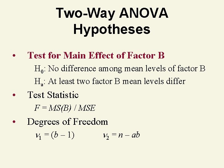
Two-Way ANOVA Hypotheses • Test for Main Effect of Factor B H 0: No difference among mean levels of factor B Ha: At least two factor B mean levels differ • Test Statistic F = MS(B) / MSE • Degrees of Freedom 1 = (b – 1) 2 = n – ab

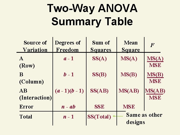
Two-Way ANOVA Summary Table Source of Variation A (Row) B (Column) Degrees of Freedom a-1 Sum of Squares SS(A) Mean Square MS(A) b-1 SS(B) MS(B) MSE SS(AB) MS(AB) MSE AB (a - 1)(b - 1) (Interaction) Error n - ab SSE Total n-1 SS(Total) F MS(A) MSE Same as other designs

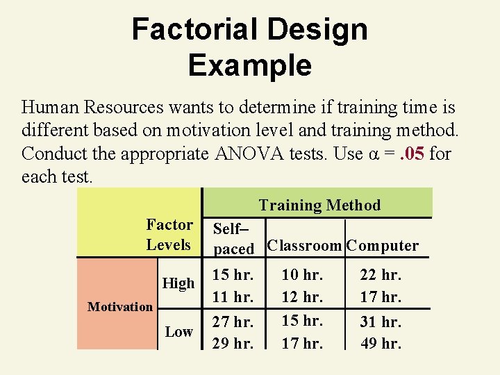
Factorial Design Example Human Resources wants to determine if training time is different based on motivation level and training method. Conduct the appropriate ANOVA tests. Use α =. 05 for each test. Training Method Factor Levels Self– paced Classroom Computer High 15 hr. 11 hr. Low 27 hr. 29 hr. Motivation 10 hr. 12 hr. 15 hr. 17 hr. 22 hr. 17 hr. 31 hr. 49 hr.

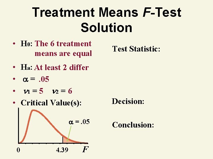
Treatment Means F-Test Solution • H 0: The 6 treatment means are equal • • Ha: At least 2 differ =. 05 1 = 5 2 = 6 Critical Value(s): =. 05 0 4. 39 F Test Statistic: Decision: Conclusion:

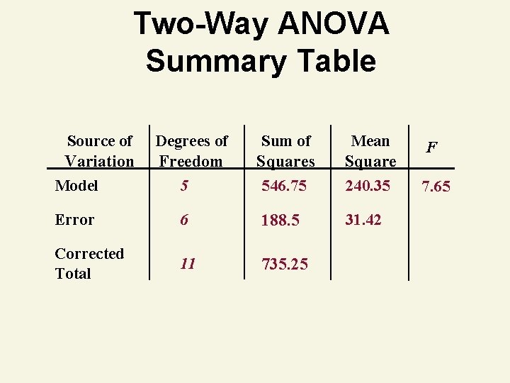
Two-Way ANOVA Summary Table Source of Variation Model Degrees of Freedom 5 Sum of Squares 546. 75 Error 6 188. 5 Corrected Total 11 735. 25 Mean Square 240. 35 31. 42 F 7. 65

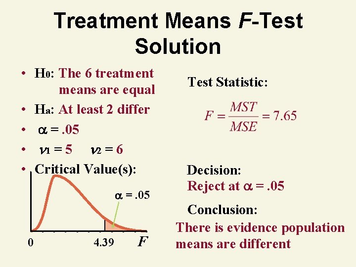
Treatment Means F-Test Solution • H 0: The 6 treatment means are equal • Ha: At least 2 differ • =. 05 • 1 = 5 2 = 6 • Critical Value(s): =. 05 0 4. 39 F Test Statistic: Decision: Reject at =. 05 Conclusion: There is evidence population means are different

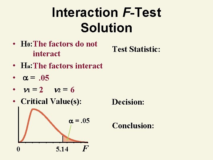
Interaction F-Test Solution • H 0: The factors do not interact • Ha: The factors interact • =. 05 • 1 = 2 2 = 6 • Critical Value(s): =. 05 0 5. 14 F Test Statistic: Decision: Conclusion:

Two-Way ANOVA Summary Table Source of Variation A (Row) Degrees of Freedom Sum of Squares Mean Square 1 546. 75 17. 40 B (Column) 2 531. 5 265. 75 8. 46 AB (Interaction) 2 123. 5 61. 76 1. 97 Error 6 188. 5 Total 11 SS(Total) 31. 42 Same as other designs F

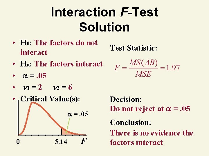
Interaction F-Test Solution • H 0: The factors do not Test Statistic: interact • Ha: The factors interact • =. 05 • 1 = 2 2 = 6 • Critical Value(s): Decision: Do not reject at =. 05 0 5. 14 F Conclusion: There is no evidence the factors interact

Main Factor A F-Test Solution • H 0: No difference between Test Statistic: motivation levels • Ha: Motivation levels differ • =. 05 • 1 = 1 2 = 6 • Critical Value(s): Decision: =. 05 0 5. 99 F Conclusion:

Two-Way ANOVA Summary Table Source of Variation A (Row) Degrees of Freedom Sum of Squares Mean Square 1 546. 75 17. 40 B (Column) 2 531. 5 265. 75 8. 46 AB (Interaction) 2 123. 5 61. 76 1. 97 Error 6 188. 5 Total 11 SS(Total) 31. 42 Same as other designs F

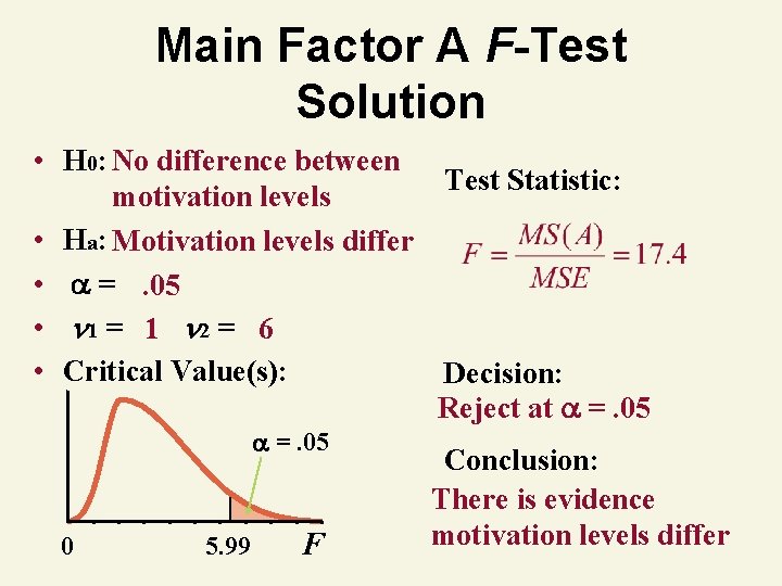
Main Factor A F-Test Solution • H 0: No difference between Test Statistic: motivation levels • Ha: Motivation levels differ • =. 05 • 1 = 1 2 = 6 • Critical Value(s): Decision: Reject at =. 05 0 5. 99 F Conclusion: There is evidence motivation levels differ

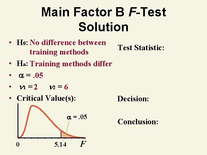
Main Factor B F-Test Solution • H 0: No difference between Test Statistic: training methods • Ha: Training methods differ • =. 05 • 1 = 2 2 = 6 • Critical Value(s): Decision: =. 05 0 5. 14 F Conclusion:

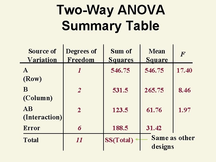
Two-Way ANOVA Summary Table Source of Variation A (Row) Degrees of Freedom Sum of Squares Mean Square 1 546. 75 17. 40 B (Column) 2 531. 5 265. 75 8. 46 AB (Interaction) 2 123. 5 61. 76 1. 97 Error 6 188. 5 Total 11 SS(Total) 31. 42 Same as other designs F

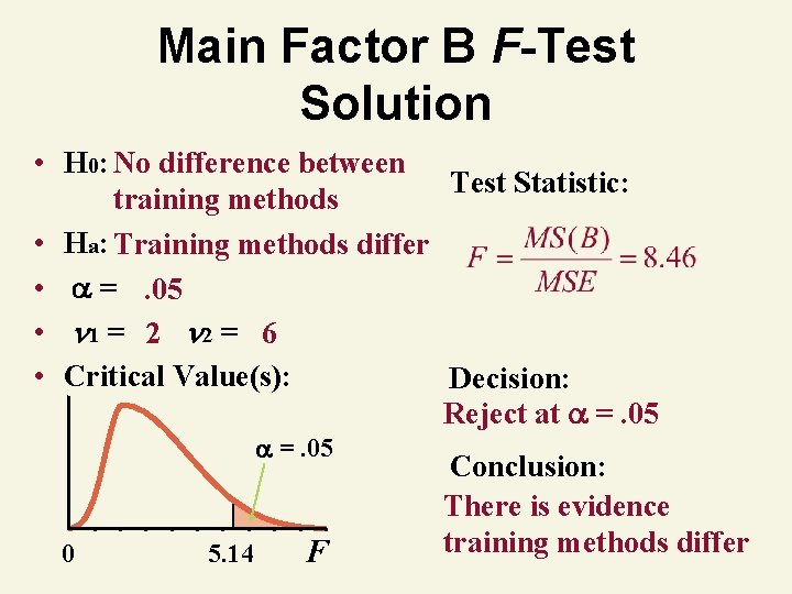
Main Factor B F-Test Solution • H 0: No difference between Test Statistic: training methods • Ha: Training methods differ • =. 05 • 1 = 2 2 = 6 • Critical Value(s): Decision: Reject at =. 05 0 5. 14 F Conclusion: There is evidence training methods differ

Conclusion 1. Described Analysis of Variance (ANOVA) 2. Explained the Rationale of ANOVA 3. Compared Experimental Designs 4. Tested the Equality of 2 or More Means • Completely Randomized Design • Factorial Design