Statistics for Business and Economics Chapter 4 Random

Statistics for Business and Economics Chapter 4 Random Variables & Probability Distributions

Learning Objectives 1. Distinguish Between the Two Types of Random Variables 2. Describe Discrete Probability Distributions 3. Describe the Uniform and Normal Distributions

Learning Objectives (continued) • Explain Sampling Distributions • Solve Probability Problems Involving Sampling Distributions

Types of Random Variables

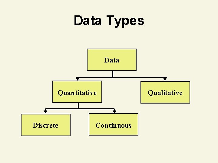
Data Types Data Quantitative Discrete Continuous Qualitative

Discrete Random Variables

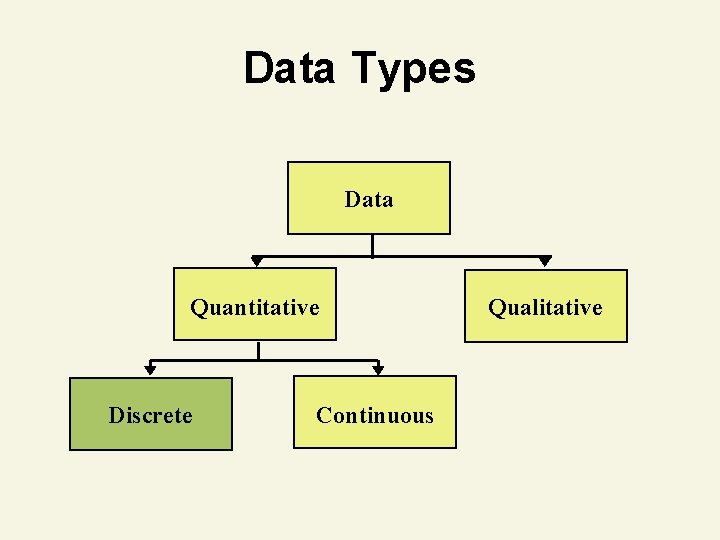
Data Types Data Quantitative Discrete Continuous Qualitative

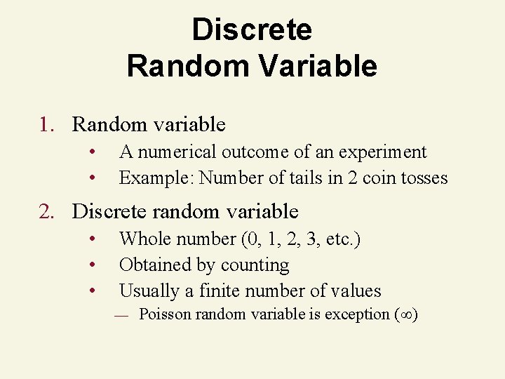
Discrete Random Variable 1. Random variable • • A numerical outcome of an experiment Example: Number of tails in 2 coin tosses 2. Discrete random variable • • • Whole number (0, 1, 2, 3, etc. ) Obtained by counting Usually a finite number of values — Poisson random variable is exception ( )

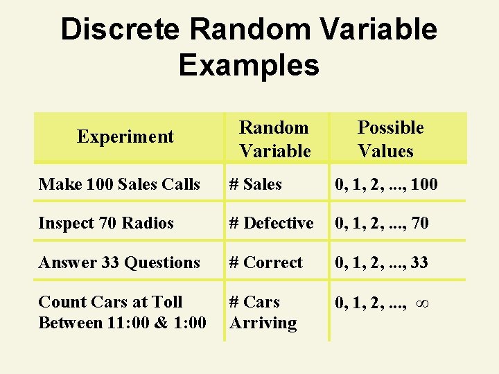
Discrete Random Variable Examples Experiment Random Variable Possible Values Make 100 Sales Calls # Sales 0, 1, 2, . . . , 100 Inspect 70 Radios # Defective 0, 1, 2, . . . , 70 Answer 33 Questions # Correct 0, 1, 2, . . . , 33 Count Cars at Toll Between 11: 00 & 1: 00 # Cars Arriving 0, 1, 2, . . . , ∞

Continuous Random Variables

Data Types Data Quantitative Discrete Continuous Qualitative

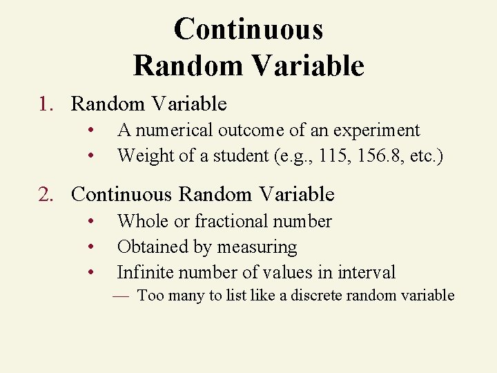
Continuous Random Variable 1. Random Variable • • A numerical outcome of an experiment Weight of a student (e. g. , 115, 156. 8, etc. ) 2. Continuous Random Variable • • • Whole or fractional number Obtained by measuring Infinite number of values in interval — Too many to list like a discrete random variable

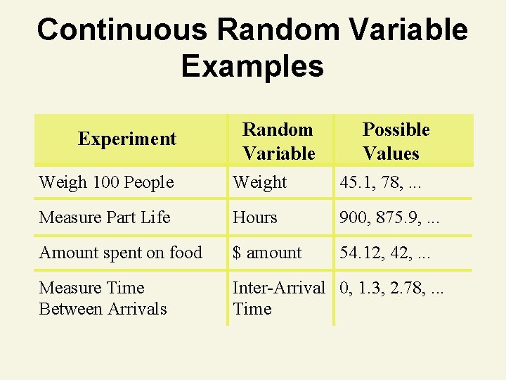
Continuous Random Variable Examples Experiment Random Variable Possible Values Weigh 100 People Weight 45. 1, 78, . . . Measure Part Life Hours 900, 875. 9, . . . Amount spent on food $ amount 54. 12, 42, . . . Measure Time Between Arrivals Inter-Arrival 0, 1. 3, 2. 78, . . . Time

Probability Distributions for Discrete Random Variables

Discrete Probability Distribution 1. List of all possible [x, p(x)] pairs • x = value of random variable (outcome) • p(x) = probability associated with value 2. Mutually exclusive (no overlap) 3. Collectively exhaustive (nothing left out) 4. 0 p(x) 1 for all x 5. p(x) = 1

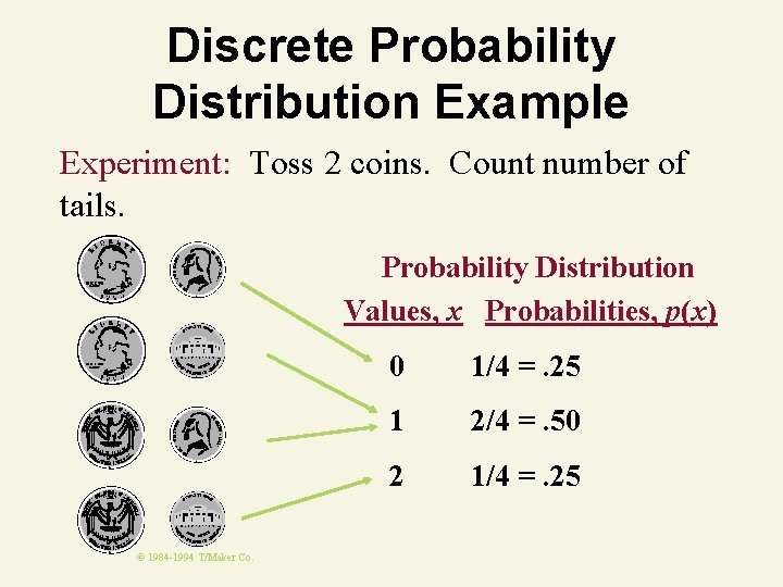
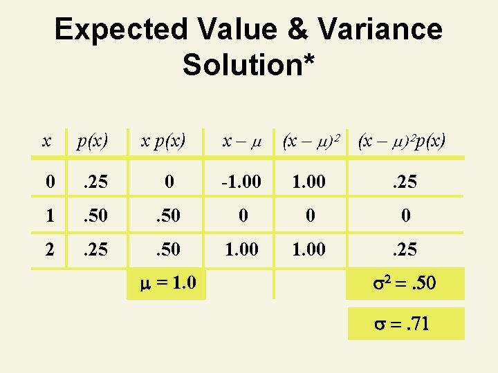
Discrete Probability Distribution Example Experiment: Toss 2 coins. Count number of tails. Probability Distribution Values, x Probabilities, p(x) © 1984 -1994 T/Maker Co. 0 1/4 =. 25 1 2/4 =. 50 2 1/4 =. 25

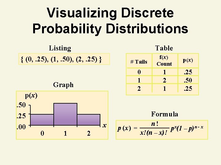
Visualizing Discrete Probability Distributions Listing Table { (0, . 25), (1, . 50), (2, . 25) } # Tails f(x) Count p(x) 0 1 2 1 . 25. 50. 25 Graph p(x). 50. 25. 00 Formula x 0 1 2 p (x ) = n! px(1 – p)n - x x!(n – x)!

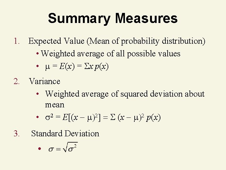
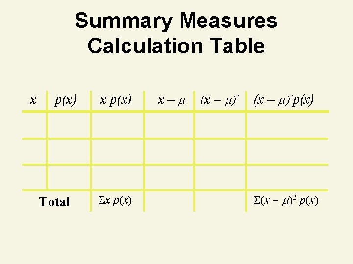
Summary Measures 1. Expected Value (Mean of probability distribution) • Weighted average of all possible values • = E(x) = x p(x) 2. Variance • Weighted average of squared deviation about mean • 2 = E[(x p(x) 3. Standard Deviation ●

Summary Measures Calculation Table x p(x) Total x p(x) x– (x – )2 p(x) (x p(x)

Thinking Challenge You toss 2 coins. You’re interested in the number of tails. What are the expected value, variance, and standard deviation of this random variable, number of tails? © 1984 -1994 T/Maker Co.

Expected Value & Variance Solution* x p(x) x– 0 . 25 0 -1. 00 . 25 1 . 50 0 0 0 2 . 25 . 50 1. 00 . 25 = 1. 0 (x – ) 2 p(x) 2 . 50 . 71

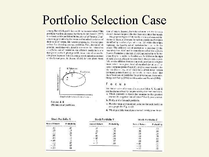
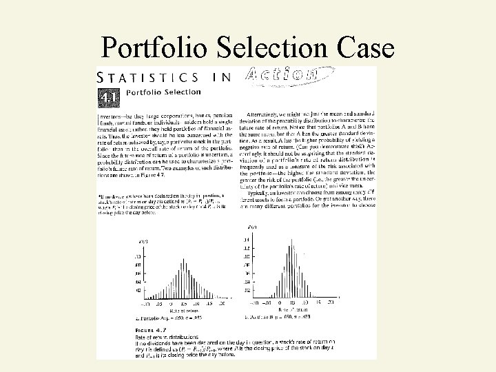
Portfolio Selection Case

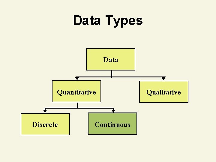
Data Types Data Quantitative Discrete Continuous Qualitative

Probability Distributions for Continuous Random Variables

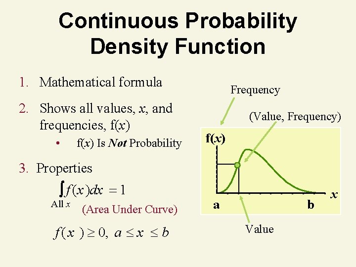
Continuous Probability Density Function 1. Mathematical formula 2. Shows all values, x, and frequencies, f(x) • f(x) Is Not Probability Frequency (Value, Frequency) f(x) 3. Properties f ( x )dx 1 All x (Area Under Curve) f ( x ) 0, a x b a b Value x

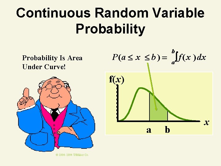
Continuous Random Variable Probability Is Area Under Curve! b P (a x b )

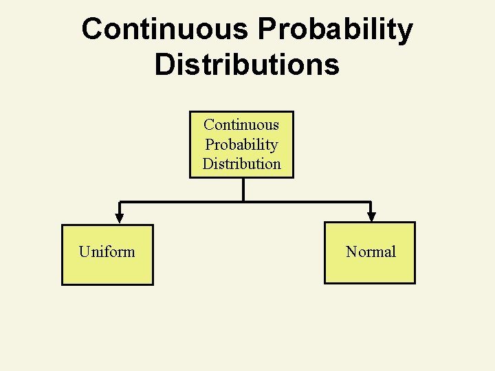
Continuous Probability Distributions Continuous Probability Distribution Uniform Normal

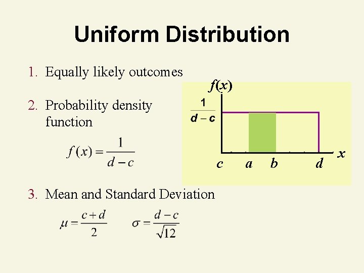
Uniform Distribution 1. Equally likely outcomes f(x) 2. Probability density function c 3. Mean and Standard Deviation a b d x

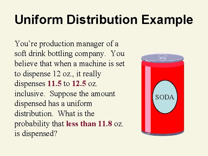
Uniform Distribution Example You’re production manager of a soft drink bottling company. You believe that when a machine is set to dispense 12 oz. , it really dispenses 11. 5 to 12. 5 oz. inclusive. Suppose the amount dispensed has a uniform distribution. What is the probability that less than 11. 8 oz. is dispensed? SODA

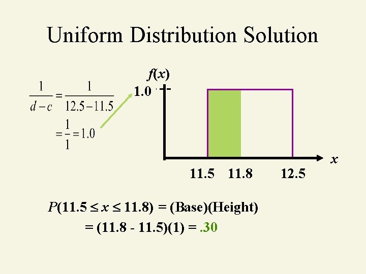
Uniform Distribution Solution f(x) 1. 0 11. 5 11. 8 P(11. 5 x 11. 8) = (Base)(Height) = (11. 8 - 11. 5)(1) =. 30 12. 5 x

Normal Distribution

Importance of Normal Distribution 1. Describes many random processes or continuous phenomena 2. Can be used to approximate discrete probability distributions • Example: binomial 3. Basis for classical statistical inference

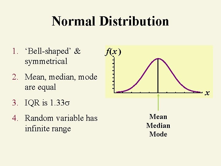
Normal Distribution 1. ‘Bell-shaped’ & symmetrical f(x ) 2. Mean, median, mode are equal x 3. IQR is 1. 33 4. Random variable has infinite range Mean Median Mode

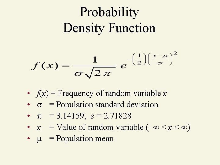
Probability Density Function • • • f(x) = Frequency of random variable x = Population standard deviation = 3. 14159; e = 2. 71828 x = Value of random variable (– < x < ) = Population mean

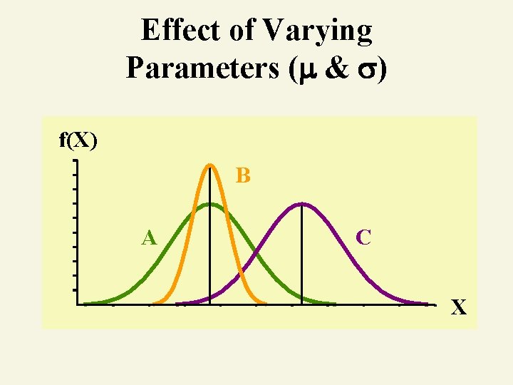
Effect of Varying Parameters ( & ) f(X) B A C X

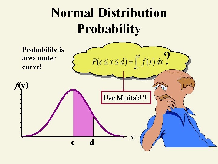
Normal Distribution Probability is area under curve! f(x) Use Minitab!!! c d x

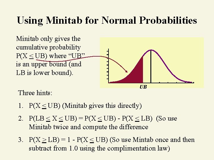
Using Minitab for Normal Probabilities Minitab only gives the cumulative probability P(X < UB) where “UB” is an upper bound (and LB is lower bound). Three hints: UB 1. P(X < UB) (Minitab gives this directly) 2. P(LB < X < UB) = P(X < UB) - P(X < LB) (So use Minitab twice and compute the difference 3. P(X > LB) = 1 - P(X < UB) (So use Mintab once and then subtract from 1. 0 using the complimentation law)

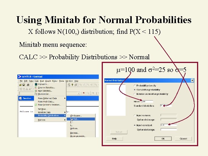
Using Minitab for Normal Probabilities X follows N(100, ) distribution; find P(X < 115) Minitab menu sequence: CALC >> Probability Distributions >> Normal =100 and 2=25 so =5

Normal Distribution Thinking Challenge You work in Quality Control for GE. Light bulb life has a normal distribution with = 2000 hours and = 200 hours. What’s the probability that a bulb will last: A. Between 2100 and 2400 hours? B. Less than 1470 hours? C. More than 2500 hours D. Greater than 2000 hours

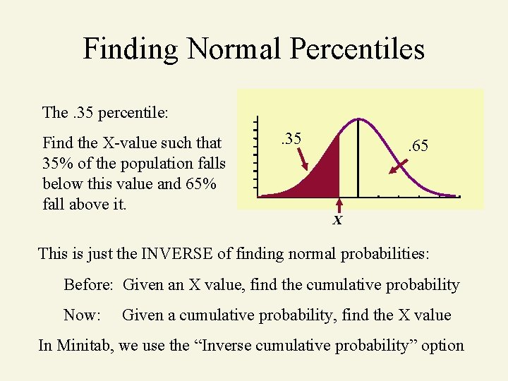
Finding Normal Percentiles The. 35 percentile: Find the X-value such that 35% of the population falls below this value and 65% fall above it. . 35 . 65 X This is just the INVERSE of finding normal probabilities: Before: Given an X value, find the cumulative probability Now: Given a cumulative probability, find the X value In Minitab, we use the “Inverse cumulative probability” option

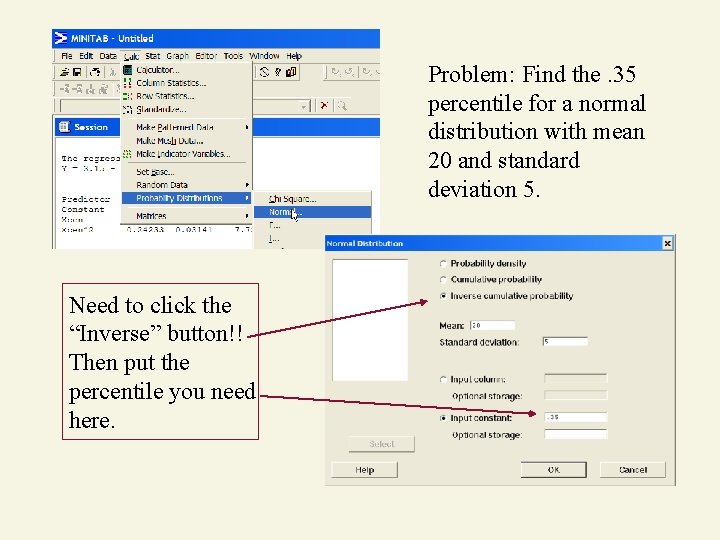
Problem: Find the. 35 percentile for a normal distribution with mean 20 and standard deviation 5. Need to click the “Inverse” button!! Then put the percentile you need here.

Reliability Example Life testing has revealed that a particular type of TV picture tube has a length of life that is approximately normally distributed with a mean of 8000 hours and a standard deviation of 1000 hours. The manufacturer wants to set a guarantee period for the tube that will obligate the manufacturer to replace no more than 5% of all tubes sold. How long should the guarantee period be?

Assessing Normality

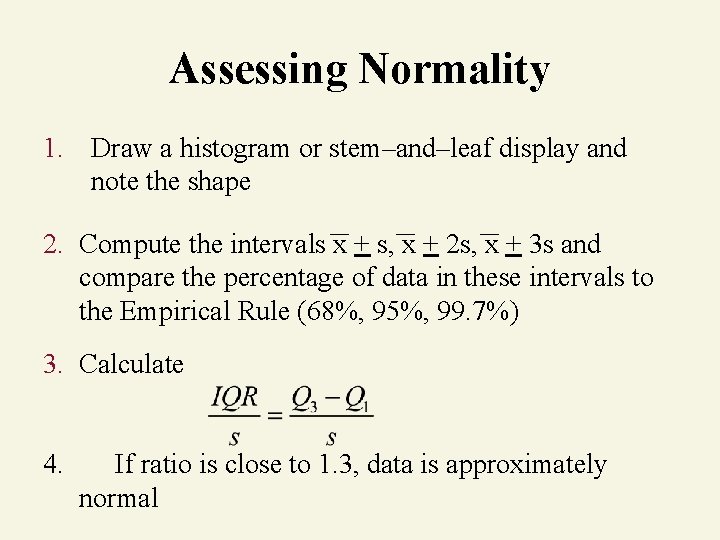
Assessing Normality 1. Draw a histogram or stem–and–leaf display and note the shape 2. Compute the intervals x + s, x + 2 s, x + 3 s and compare the percentage of data in these intervals to the Empirical Rule (68%, 95%, 99. 7%) 3. Calculate 4. If ratio is close to 1. 3, data is approximately normal

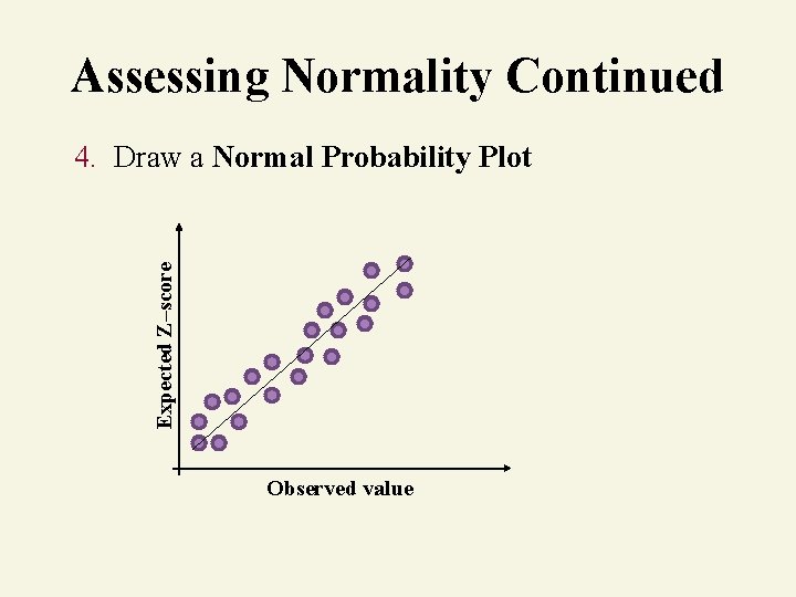
Assessing Normality Continued Expected Z–score 4. Draw a Normal Probability Plot Observed value

Checking for Normality Construct a “normal probability plot” of the data. If the data are approximately normal, the points will fall approximately on a straight line. _ Suppose the sample has mean X and standard deviation s. Then the normal probability plots: X Axis: Actual value (and suppose its percentile is p) Y Axis: The pth percentile from_an actual normal distribution with mean X and standard deviation s (i. e. , the “expected normal value”)

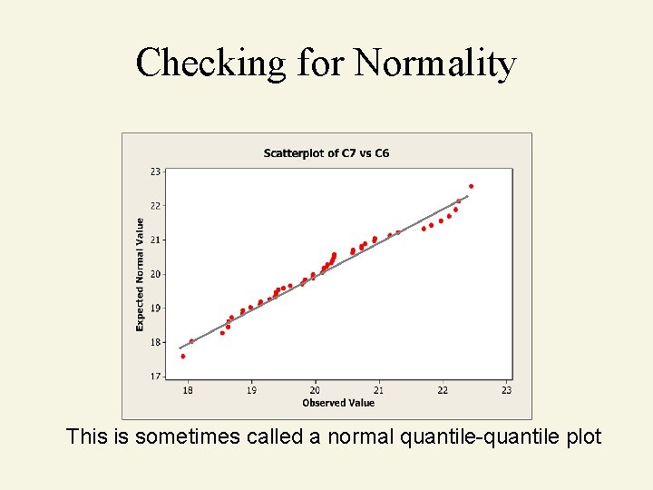
Checking for Normality This is sometimes called a normal quantile-quantile plot

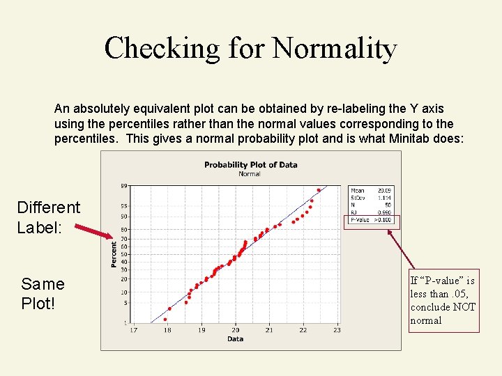
Checking for Normality An absolutely equivalent plot can be obtained by re-labeling the Y axis using the percentiles rather than the normal values corresponding to the percentiles. This gives a normal probability plot and is what Minitab does: Different Label: Same Plot! If “P-value” is less than. 05, conclude NOT normal

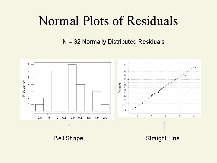
Normal Plots of Residuals N = 32 Normally Distributed Residuals Bell Shape Straight Line

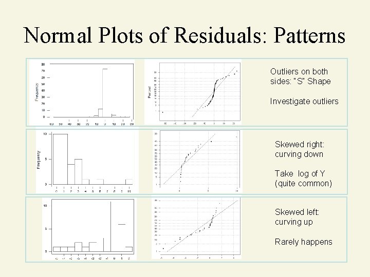
Normal Plots of Residuals: Patterns Outliers on both sides: “S” Shape Investigate outliers Skewed right: curving down Take log of Y (quite common) Skewed left: curving up Rarely happens

Sampling Distributions

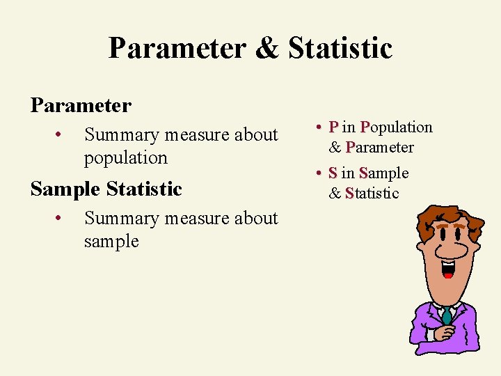
Parameter & Statistic Parameter • Summary measure about population Sample Statistic • Summary measure about sample • P in Population & Parameter • S in Sample & Statistic

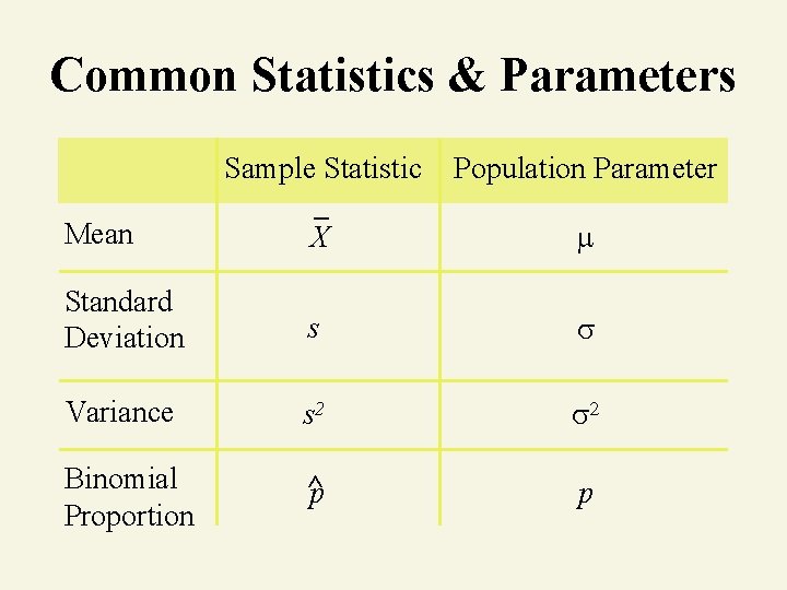
Common Statistics & Parameters Sample Statistic Population Parameter Mean X Standard Deviation s Variance s 2 Binomial Proportion ^ p p

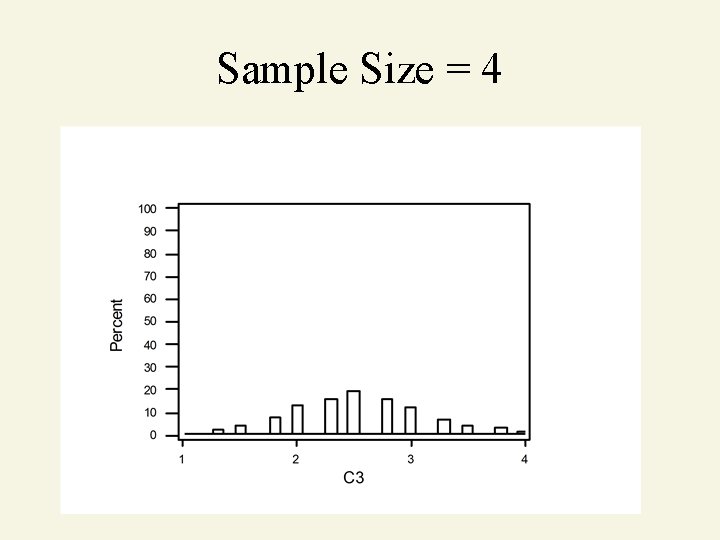
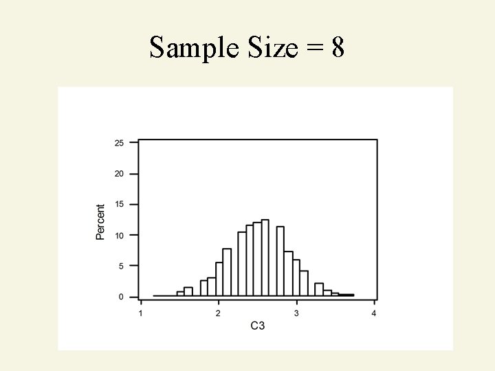
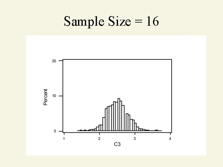
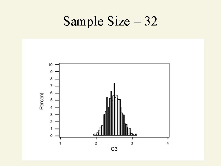
Sampling Distribution 1. Theoretical probability distribution 2. Random variable is sample statistic • Sample mean, sample proportion, etc. 3. Results from drawing all possible samples of a fixed size 4. List of all possible [x, p(x)] pairs • Sampling distribution of the sample mean

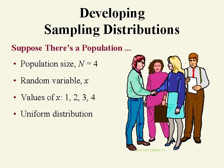
Developing Sampling Distributions Suppose There’s a Population. . . • Population size, N =

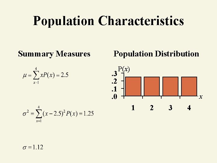
Population Characteristics Summary Measures Population Distribution. 3. 2. 1. 0 P(x) x 1 2 3 4

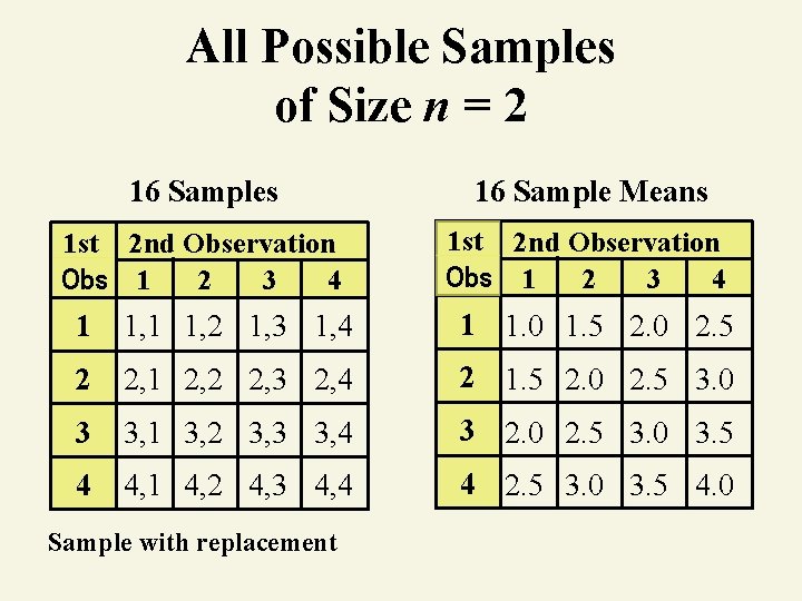
All Possible Samples of Size n = 2 16 Samples 16 Sample Means 1 st 2 nd Observation Obs 1 2 3 4 1 1, 2 1, 3 1, 4 1 1. 0 1. 5 2. 0 2. 5 2 2, 1 2, 2 2, 3 2, 4 2 1. 5 2. 0 2. 5 3. 0 3 3, 1 3, 2 3, 3 3, 4 3 2. 0 2. 5 3. 0 3. 5 4 4, 1 4, 2 4, 3 4, 4 4 2. 5 3. 0 3. 5 4. 0 Sample with replacement

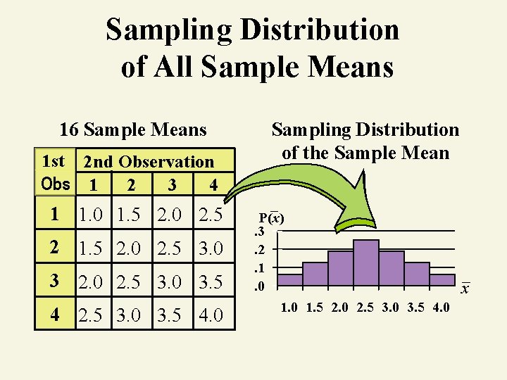
Sampling Distribution of All Sample Means 16 Sample Means 1 st 2 nd Observation Obs 1 2 3 4 1 1. 0 1. 5 2. 0 2. 5 2 1. 5 2. 0 2. 5 3. 0 3. 5 4. 0 Sampling Distribution of the Sample Mean P(x). 3. 2. 1. 0 1. 5 2. 0 2. 5 3. 0 3. 5 4. 0 x

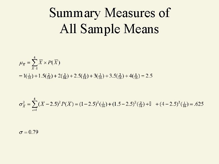
Summary Measures of All Sample Means

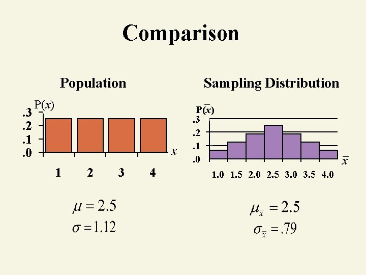
Comparison Population. 3. 2. 1. 0 Sampling Distribution P(x) x 1 2 3 4 P(x). 3. 2. 1. 0 1. 5 2. 0 2. 5 3. 0 3. 5 4. 0 x

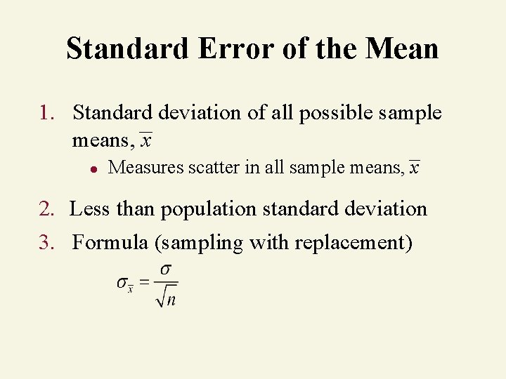
Standard Error of the Mean 1. Standard deviation of all possible sample means, x ● Measures scatter in all sample means, x 2. Less than population standard deviation 3. Formula (sampling with replacement)

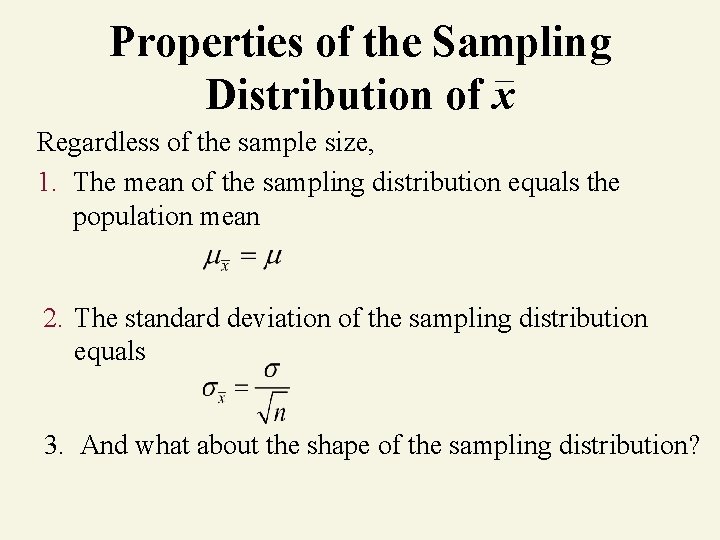
Properties of the Sampling Distribution of x Regardless of the sample size, 1. The mean of the sampling distribution equals the population mean 2. The standard deviation of the sampling distribution equals 3. And what about the shape of the sampling distribution?

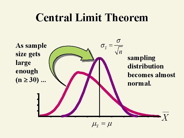
Central Limit Theorem As sample size gets large enough (n 30). . . sampling distribution becomes almost normal. X

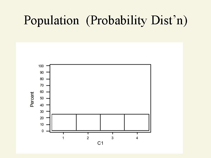
Population (Probability Dist’n)

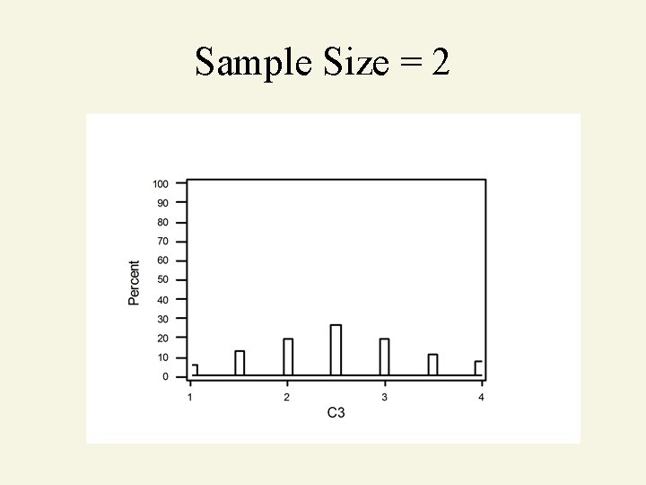
Sample Size = 2

Sample Size = 4

Sample Size = 8

Sample Size = 16

Sample Size = 32

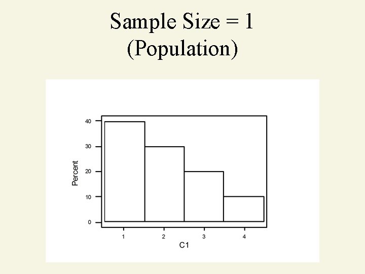
Sample Size = 1 (Population)

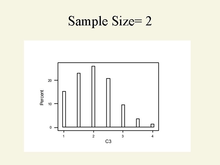
Sample Size= 2

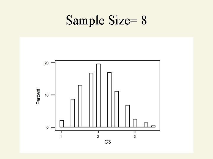
Sample Size= 8

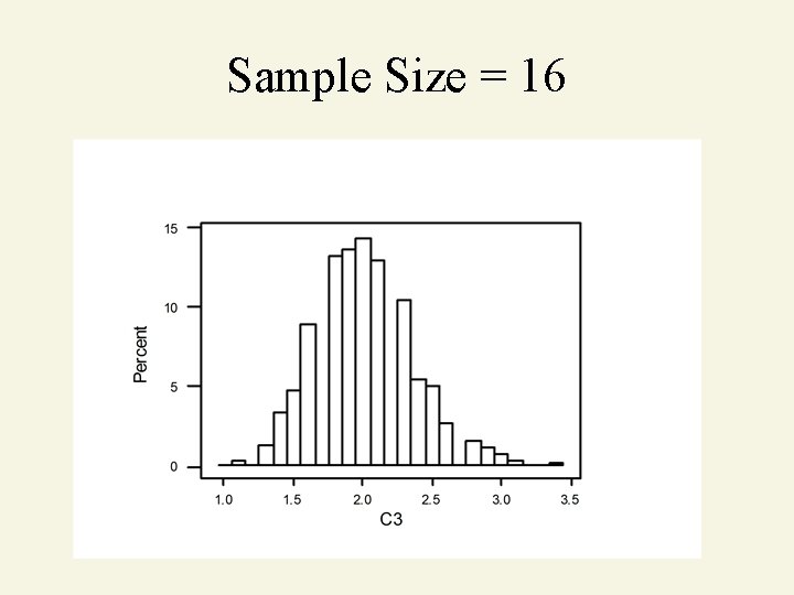
Sample Size = 16

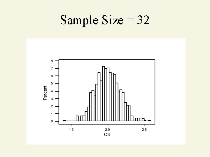
Sample Size = 32

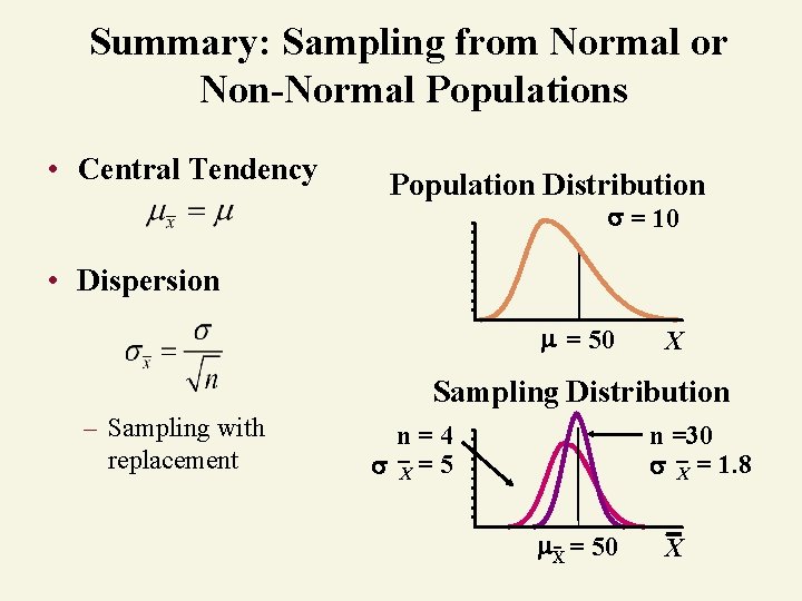
Summary: Sampling from Normal or Non-Normal Populations • Central Tendency Population Distribution = 10 • Dispersion = 50 X Sampling Distribution – Sampling with replacement n=4 X = 5 n =30 X = 1. 8 X- = 50 X

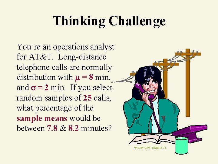
Thinking Challenge You’re an operations analyst for AT&T. Long-distance telephone calls are normally distribution with = 8 min. and = 2 min. If you select random samples of 25 calls, what percentage of the sample means would be between 7. 8 & 8. 2 minutes? © 1984 -1994 T/Maker Co.

Central Limit Theorem Example The amount of soda in cans of a particular brand has a mean of 12 oz and a standard deviation of. 2 oz. If you select random samples of 50 cans, what percentage of the sample means would be less than 11. 95 oz? SODA

Conclusion 1. Distinguished Between the Two Types of Random Variables 2. Described Discrete Probability Distributions 3. Described the Uniform and Normal Distributions 4. Explained Sampling Distributions 5. Solved Probability Problems Involving Sampling Distributions