Statistics for Business and Economics 7 th Edition

Chapter Goals After completing this chapter, you should be able to: n Recognize situations in which to use analysis of variance n Understand different analysis of variance designs n n n Perform a one-way and two-way analysis of variance and interpret the results Conduct and interpret a Kruskal-Wallis test Analyze two-factor analysis of variance tests with more than one observation per cell Copyright © 2010 Pearson Education, Inc. Publishing as Prentice Hall Ch. 15 -2

15. 2 n One-Way Analysis of Variance Evaluate the difference among the means of three or more groups Examples: Average production for 1 st, 2 nd, and 3 rd shifts Expected mileage for five brands of tires n Assumptions n Populations are normally distributed n Populations have equal variances n Samples are randomly and independently drawn Copyright © 2010 Pearson Education, Inc. Publishing as Prentice Hall Ch. 15 -3

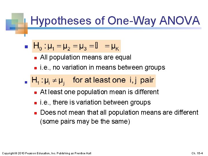
Hypotheses of One-Way ANOVA n n n All population means are equal n i. e. , no variation in means between groups n At least one population mean is different n i. e. , there is variation between groups n Does not mean that all population means are different (some pairs may be the same) Copyright © 2010 Pearson Education, Inc. Publishing as Prentice Hall Ch. 15 -4

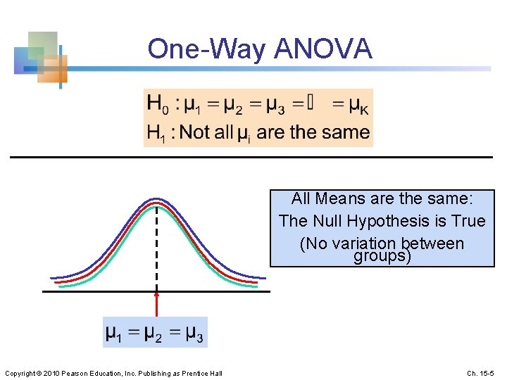
One-Way ANOVA All Means are the same: The Null Hypothesis is True (No variation

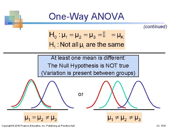
One-Way ANOVA (continued) At least one mean is different: The Null Hypothesis is NOT true (Variation is present between groups) or Copyright © 2010 Pearson Education, Inc. Publishing as Prentice Hall Ch. 15 -6

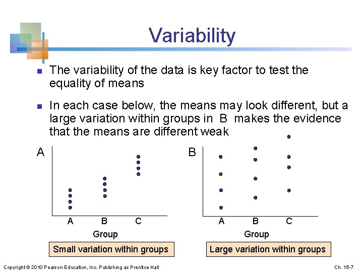
Variability n n The variability of the data is key factor to test the equality of means In each case below, the means may look different, but a large variation within groups in B makes the evidence that the means are different weak A B A B C Group Small variation within groups Copyright © 2010 Pearson Education, Inc. Publishing as Prentice Hall A B C Group Large variation within groups Ch. 15 -7

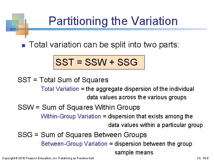
Partitioning the Variation n Total variation can be split into two parts: SST = SSW + SSG SST = Total Sum of Squares Total Variation = the aggregate dispersion of the individual data values across the various groups SSW = Sum of Squares Within Groups Within-Group Variation = dispersion that exists among the data values within a particular group SSG = Sum of Squares Between Groups Between-Group Variation = dispersion between the group sample means Copyright © 2010 Pearson Education, Inc. Publishing as Prentice Hall Ch. 15 -8

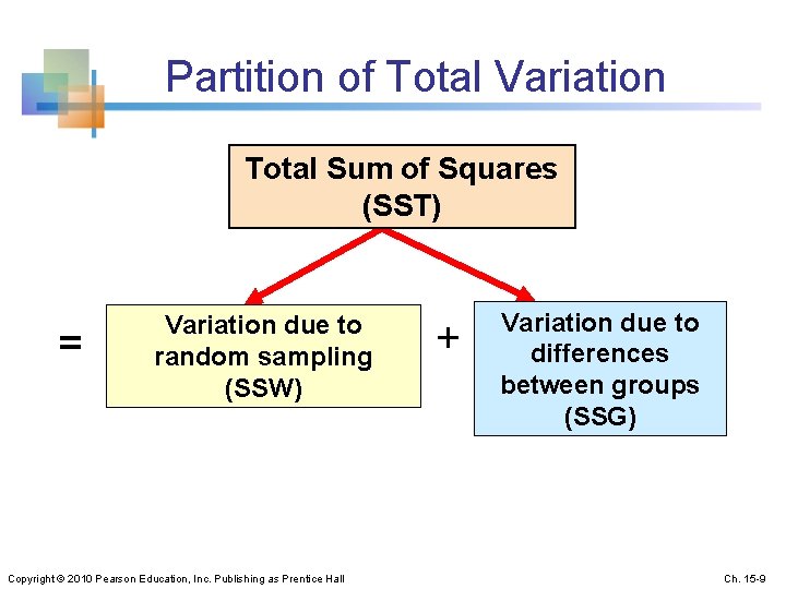
Partition of Total Variation Total Sum of Squares (SST) = Variation due to random sampling (SSW) Copyright © 2010 Pearson Education, Inc. Publishing as Prentice Hall + Variation due to differences between groups (SSG) Ch. 15 -9

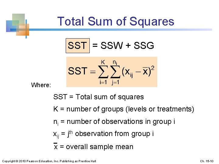
Total Sum of Squares SST = SSW + SSG Where: SST = Total sum of squares K = number of groups (levels or treatments) ni = number of observations in group i xij = jth observation from group i x = overall sample mean Copyright © 2010 Pearson Education, Inc. Publishing as Prentice Hall Ch. 15 -10

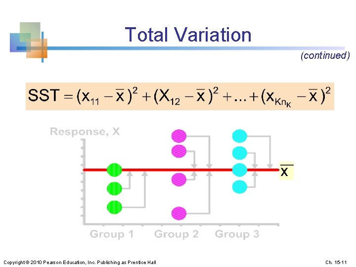
Total Variation (continued) Copyright © 2010 Pearson Education, Inc. Publishing as Prentice Hall Ch.

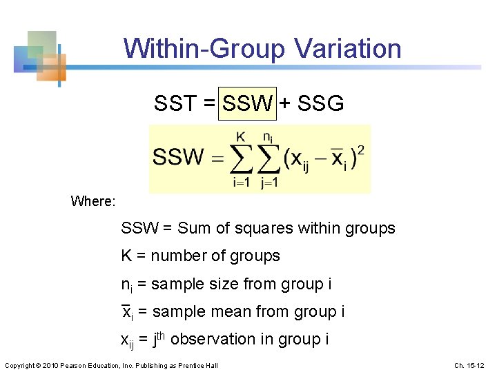
Within-Group Variation SST = SSW + SSG Where: SSW = Sum of squares within groups K = number of groups ni = sample size from group i xi = sample mean from group i xij = jth observation in group i Copyright © 2010 Pearson Education, Inc. Publishing as Prentice Hall Ch. 15 -12

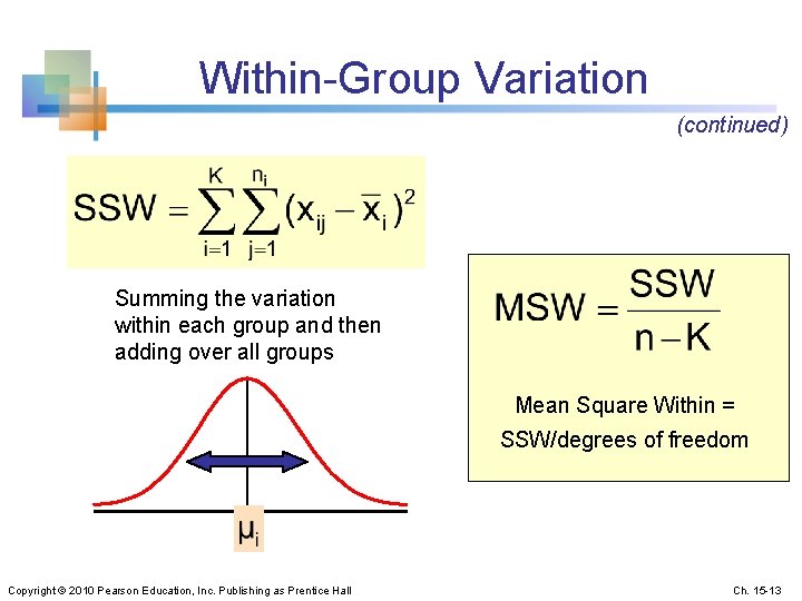
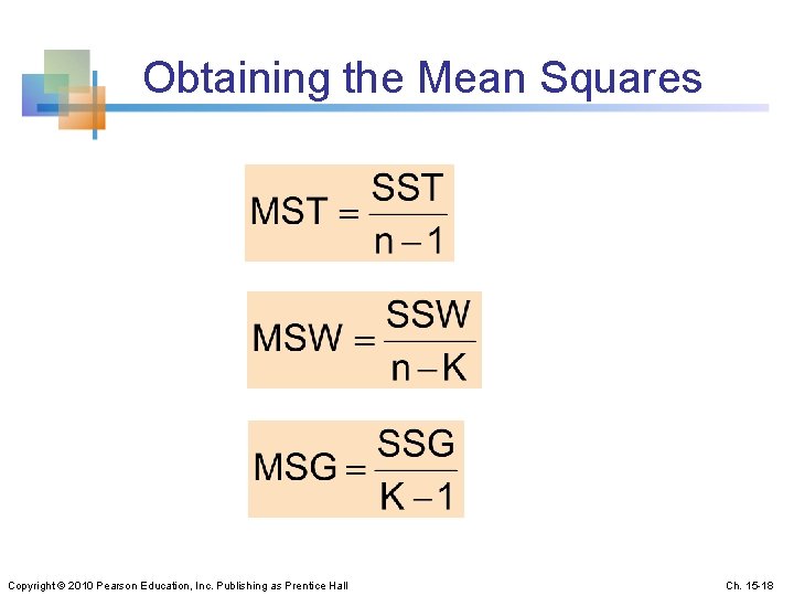
Within-Group Variation (continued) Summing the variation within each group and then adding over all groups Mean Square Within = SSW/degrees of freedom Copyright © 2010 Pearson Education, Inc. Publishing as Prentice Hall Ch. 15 -13

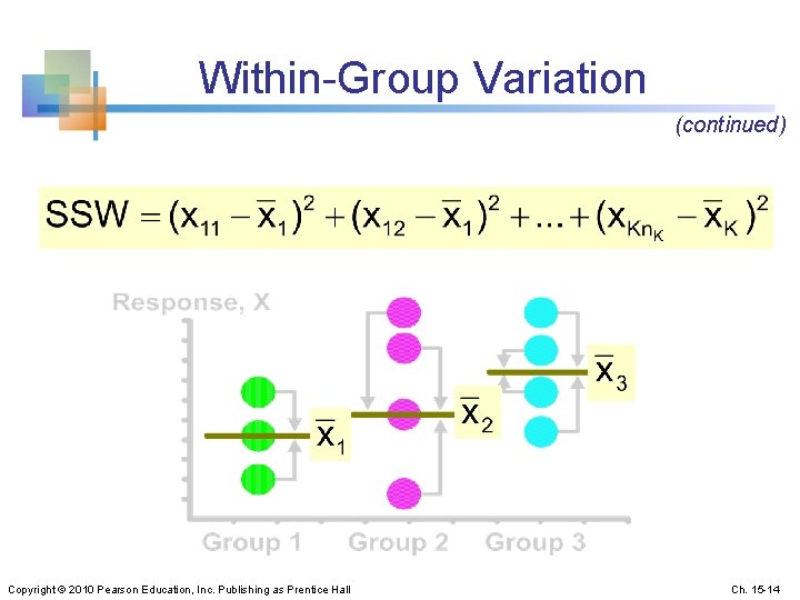
Within-Group Variation (continued) Copyright © 2010 Pearson Education, Inc. Publishing as Prentice Hall Ch.

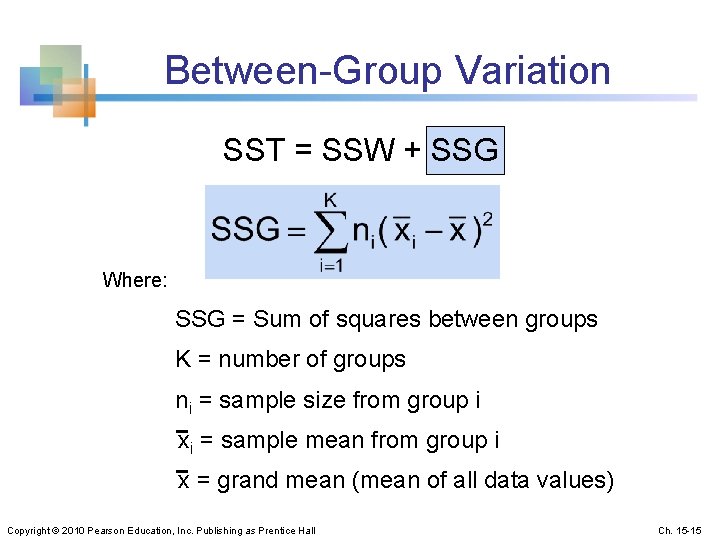
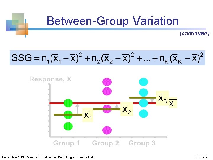
Between-Group Variation SST = SSW + SSG Where: SSG = Sum of squares between groups K = number of groups ni = sample size from group i xi = sample mean from group i x = grand mean (mean of all data values) Copyright © 2010 Pearson Education, Inc. Publishing as Prentice Hall Ch. 15 -15

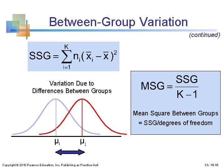
Between-Group Variation (continued) Variation Due to Differences Between Groups Mean Square Between Groups = SSG/degrees of freedom Copyright © 2010 Pearson Education, Inc. Publishing as Prentice Hall Ch. 15 -16

Between-Group Variation (continued) Copyright © 2010 Pearson Education, Inc. Publishing as Prentice Hall Ch.

Obtaining the Mean Squares Copyright © 2010 Pearson Education, Inc. Publishing as Prentice Hall

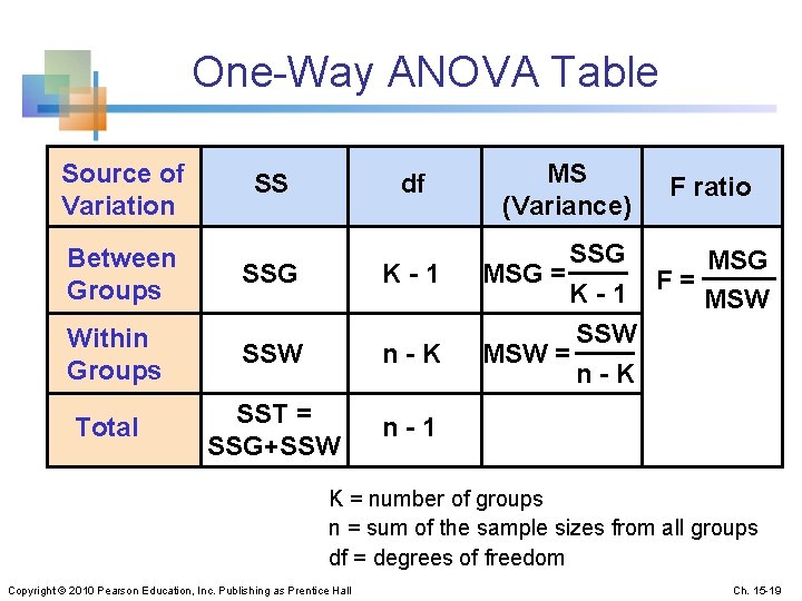
One-Way ANOVA Table Source of Variation SS df Between Groups SSG K-1 Within Groups SSW n-K Total SST = SSG+SSW n-1 MS (Variance) F ratio SSG MSG = K - 1 F = MSW SSW MSW = n-K K = number of groups n = sum of the sample sizes from all groups df = degrees of freedom Copyright © 2010 Pearson Education, Inc. Publishing as Prentice Hall Ch. 15 -19

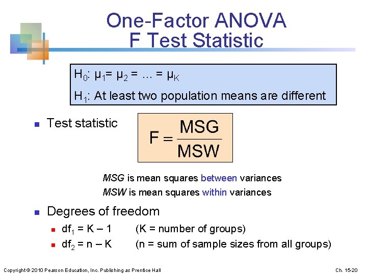
One-Factor ANOVA F Test Statistic H 0: μ 1= μ 2 = … = μK H 1: At least two population means are different n Test statistic MSG is mean squares between variances MSW is mean squares within variances n Degrees of freedom n n df 1 = K – 1 (K = number of groups) df 2 = n – K (n = sum of sample sizes from all groups) Copyright © 2010 Pearson Education, Inc. Publishing as Prentice Hall Ch. 15 -20

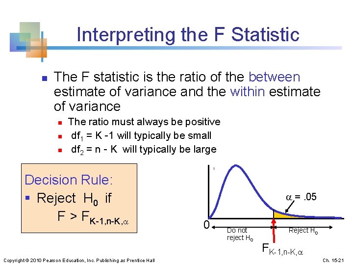
Interpreting the F Statistic n The F statistic is the ratio of the between estimate of variance and the within estimate of variance n n n The ratio must always be positive df 1 = K -1 will typically be small df 2 = n - K will typically be large Decision Rule: § Reject H 0 if F > FK-1, n-K, Copyright © 2010 Pearson Education, Inc. Publishing as Prentice Hall =. 05 0 Do not reject H 0 Reject H 0 FK-1, n-K, Ch. 15 -21

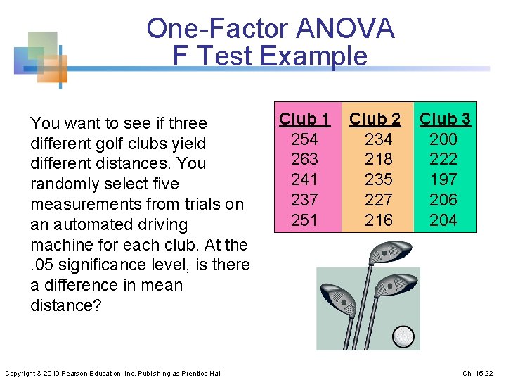
One-Factor ANOVA F Test Example You want to see if three different golf clubs yield different distances. You randomly select five measurements from trials on an automated driving machine for each club. At the . 05 significance level, is there a difference in mean distance? Copyright © 2010 Pearson Education, Inc. Publishing as Prentice Hall Club 1 Club 2 Club 3 254 234 200 263 218 222 241 235 197 237 227 206 251 216 204 Ch. 15 -22

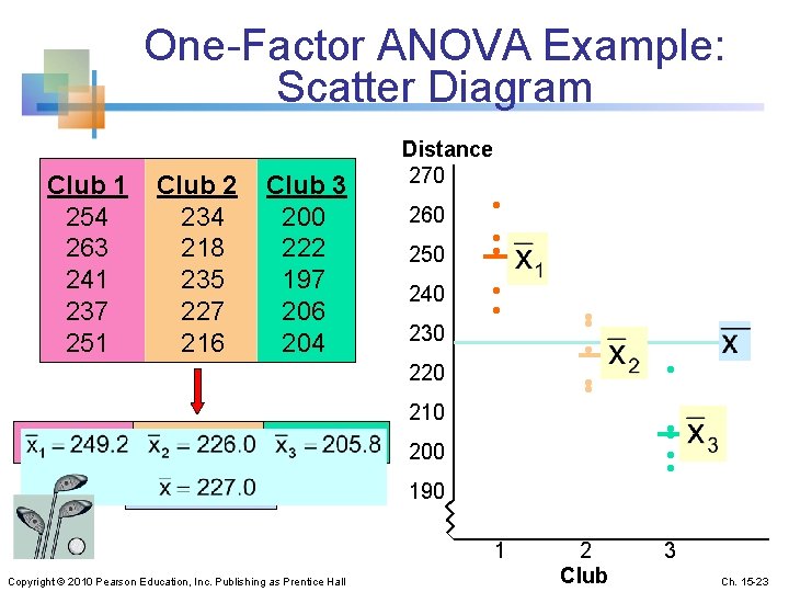
One-Factor ANOVA Example: Scatter Diagram Club 1 Club 2 Club 3 254 234 200 263 218 222 241 235 197 237 227 206 251 216 204 Distance 270 260 250 240 230 220 210 200 190 Copyright © 2010 Pearson Education, Inc. Publishing as Prentice Hall • • • • • 1 2 3 Club Ch. 15 -23

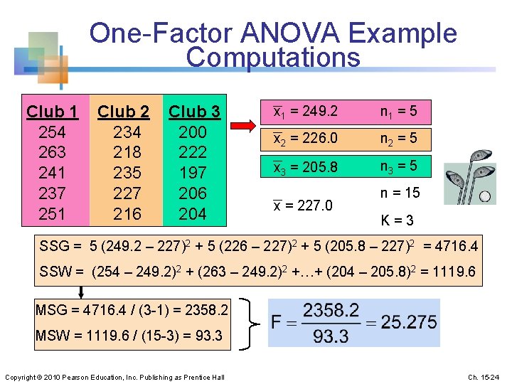
One-Factor ANOVA Example Computations Club 1 Club 2 Club 3 254 234 200 263 218 222 241 235 197 237 227 206 251 216 204 x 1 = 249. 2 n 1 = 5 x 2 = 226. 0 n 2 = 5 x 3 = 205. 8 n 3 = 5 x = 227. 0 n = 15 K = 3 SSG = 5 (249. 2 – 227)2 + 5 (226 – 227)2 + 5 (205. 8 – 227)2 = 4716. 4 SSW = (254 – 249. 2)2 + (263 – 249. 2)2 +…+ (204 – 205. 8)2 = 1119. 6 MSG = 4716. 4 / (3 -1) = 2358. 2 MSW = 1119. 6 / (15 -3) = 93. 3 Copyright © 2010 Pearson Education, Inc. Publishing as Prentice Hall Ch. 15 -24

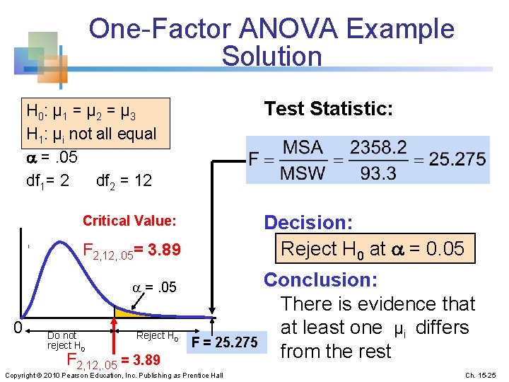
One-Factor ANOVA Example Solution Test Statistic: H 0: μ 1 = μ 2 = μ 3 H 1: μi not all equal =. 05 df 1= 2 df 2 = 12 Decision: Reject H 0 at = 0. 05 Critical Value: F 2, 12, . 05= 3. 89 =. 05 0 Do not reject H 0 Reject H 0 F 2, 12, . 05 = 3. 89 Conclusion: There is evidence that at least one μi differs F = 25. 275 from the rest Copyright © 2010 Pearson Education, Inc. Publishing as Prentice Hall Ch. 15 -25

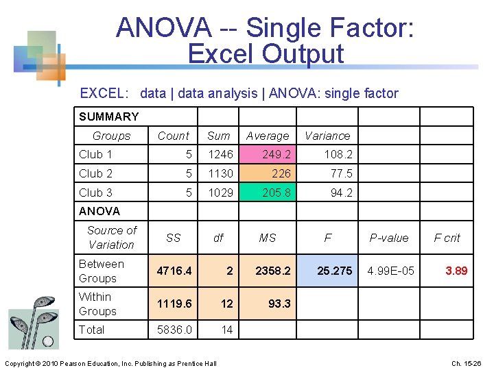
ANOVA -- Single Factor: Excel Output EXCEL: data | data analysis | ANOVA: single factor SUMMARY Groups Count Sum Average Variance Club 1 5 1246 249. 2 108. 2 Club 2 5 1130 226 77. 5 Club 3 5 1029 205. 8 94. 2 ANOVA Source of Variation SS df MS Between Groups 4716. 4 2 2358. 2 Within Groups 1119. 6 12 93. 3 Total 5836. 0 14 Copyright © 2010 Pearson Education, Inc. Publishing as Prentice Hall F P-value 25. 275 F crit 4. 99 E-05 3. 89 Ch. 15 -26

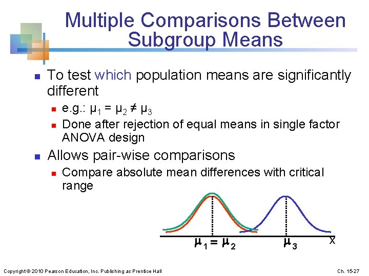
Multiple Comparisons Between Subgroup Means n To test which population means are significantly different n n n e. g. : μ 1 = μ 2 ≠ μ 3 Done after rejection of equal means in single factor ANOVA design Allows pair-wise comparisons n Compare absolute mean differences with critical range 1= 2 Copyright © 2010 Pearson Education, Inc. Publishing as Prentice Hall 3 x Ch. 15 -27

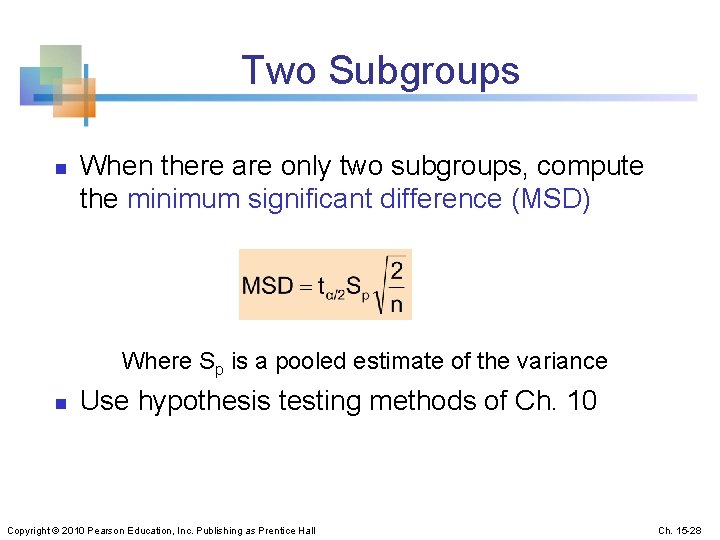
Two Subgroups n When there are only two subgroups, compute the minimum significant difference (MSD) Where Sp is a pooled estimate of the variance n Use hypothesis testing methods of Ch. 10 Copyright © 2010 Pearson Education, Inc. Publishing as Prentice Hall Ch. 15 -28

Multiple Supgroups n The minimum significant difference between k subgroups is where § q is a factor from appendix Table 13 for the chosen level of § k = number of subgroups, and § MSW = Mean square within from ANOVA table Copyright © 2010 Pearson Education, Inc. Publishing as Prentice Hall Ch. 15 -29

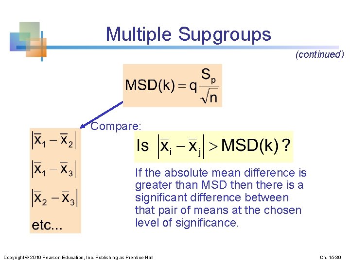
Multiple Supgroups (continued) Compare: If the absolute mean difference is greater than MSD then there is a significant difference between that pair of means at the chosen level of significance. Copyright © 2010 Pearson Education, Inc. Publishing as Prentice Hall Ch. 15 -30

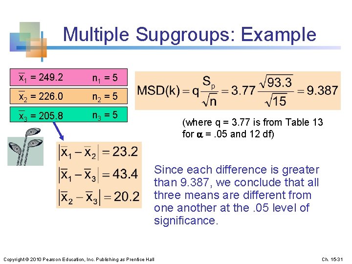
Multiple Supgroups: Example x 1 = 249. 2 n 1 = 5 x 2 = 226. 0 n 2 = 5 x 3 = 205. 8 n 3 = 5 (where q = 3. 77 is from Table 13 for =. 05 and 12 df) Since each difference is greater than 9. 387, we conclude that all three means are different from one another at the. 05 level of significance. Copyright © 2010 Pearson Education, Inc. Publishing as Prentice Hall Ch. 15 -31

15. 3 n n Kruskal-Wallis Test Use when the normality assumption for one-way ANOVA is violated Assumptions: n n n The samples are random and independent variables have a continuous distribution the data can be ranked populations have the same variability populations have the same shape Copyright © 2010 Pearson Education, Inc. Publishing as Prentice Hall Ch. 15 -32

Kruskal-Wallis Test Procedure n Obtain relative rankings for each value n n In event of tie, each of the tied values gets the average rank Sum the rankings for data from each of the K groups n n Compute the Kruskal-Wallis test statistic Evaluate using the chi-square distribution with K – 1 degrees of freedom Copyright © 2010 Pearson Education, Inc. Publishing as Prentice Hall Ch. 15 -33

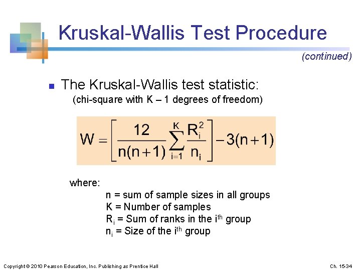
Kruskal-Wallis Test Procedure (continued) n The Kruskal-Wallis test statistic: (chi-square with K – 1 degrees of freedom) where: n = sum of sample sizes in all groups K = Number of samples Ri = Sum of ranks in the ith group ni = Size of the ith group Copyright © 2010 Pearson Education, Inc. Publishing as Prentice Hall Ch. 15 -34

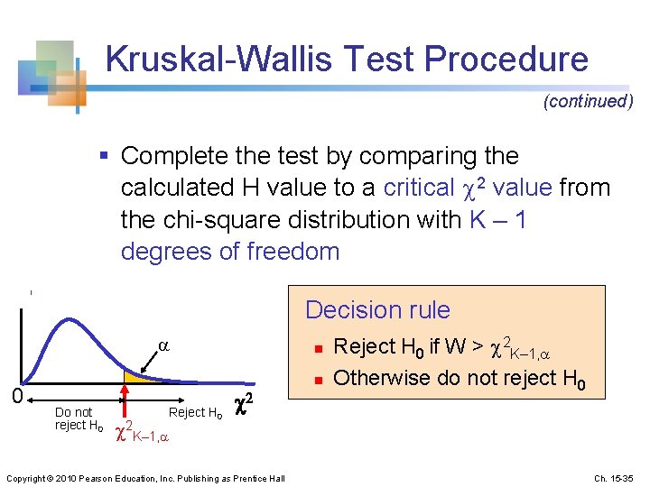
Kruskal-Wallis Test Procedure (continued) § Complete the test by comparing the calculated H value to a critical 2 value from the chi-square distribution with K – 1 degrees of freedom Decision rule 0 Do not reject H 0 2 K– 1, Reject H 0 n 2 Copyright © 2010 Pearson Education, Inc. Publishing as Prentice Hall n Reject H 0 if W > 2 K– 1, Otherwise do not reject H 0 Ch. 15 -35

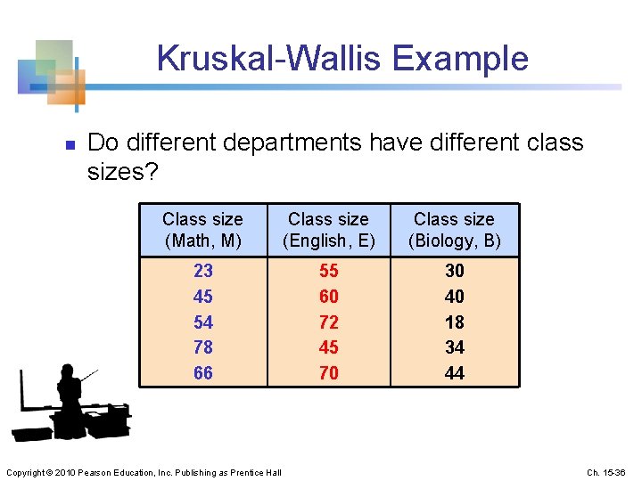
Kruskal-Wallis Example n Do different departments have different class sizes? Class size (Math, M) Class size (English, E) Class size (Biology, B) 23 45 54 78 66 55 60 72 45 70 30 40 18 34 44 Copyright © 2010 Pearson Education, Inc. Publishing as Prentice Hall Ch. 15 -36

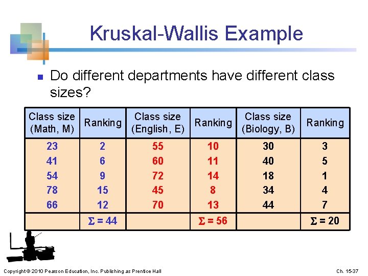
Kruskal-Wallis Example n Do different departments have different class sizes? Class size Ranking (Math, M) (English, E) (Biology, B) 23 41 54 78 66 2 6 9 15 12 55 60 72 45 70 = 44 Copyright © 2010 Pearson Education, Inc. Publishing as Prentice Hall 10 11 14 8 13 = 56 30 40 18 34 44 Ranking 3 5 1 4 7 = 20 Ch. 15 -37

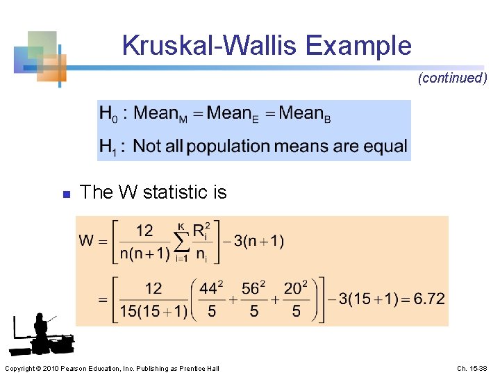
Kruskal-Wallis Example (continued) n The W statistic is Copyright © 2010 Pearson Education, Inc.

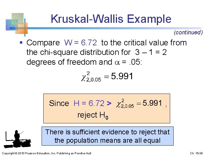
Kruskal-Wallis Example (continued) § Compare W = 6. 72 to the critical value from the chi-square distribution for 3 – 1 = 2 degrees of freedom and =. 05: Since H = 6. 72 > , reject H 0 There is sufficient evidence to reject that the population means are all equal Copyright © 2010 Pearson Education, Inc. Publishing as Prentice Hall Ch. 15 -39

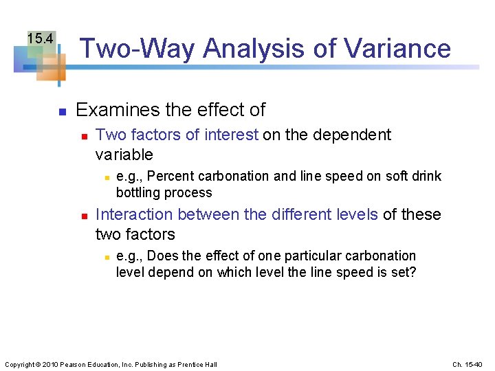
15. 4 Two-Way Analysis of Variance n Examines the effect of n Two factors of interest on the dependent variable n n e. g. , Percent carbonation and line speed on soft drink bottling process Interaction between the different levels of these two factors n e. g. , Does the effect of one particular carbonation level depend on which level the line speed is set? Copyright © 2010 Pearson Education, Inc. Publishing as Prentice Hall Ch. 15 -40

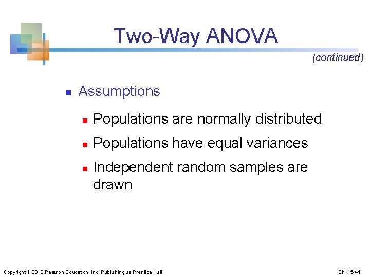
Two-Way ANOVA (continued) n Assumptions n Populations are normally distributed n Populations have equal variances n Independent random samples are drawn Copyright © 2010 Pearson Education, Inc. Publishing as Prentice Hall Ch. 15 -41

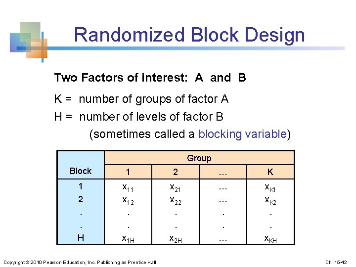
Randomized Block Design Two Factors of interest: A and B K = number of groups of factor A H = number of levels of factor B (sometimes called a blocking variable) Group Block 1 2 … K 1 2. . H x 11 x 12. . x 1 H x 21 x 22. . x 2 H … …. . … x. K 1 x. K 2. . x. KH Copyright © 2010 Pearson Education, Inc. Publishing as Prentice Hall Ch. 15 -42

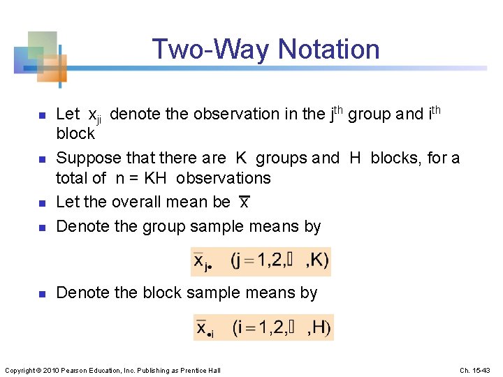
Two-Way Notation n Let xji denote the observation in the jth group and ith block Suppose that there are K groups and H blocks, for a total of n = KH observations Let the overall mean be x Denote the group sample means by n Denote the block sample means by n n n Copyright © 2010 Pearson Education, Inc. Publishing as Prentice Hall Ch. 15 -43

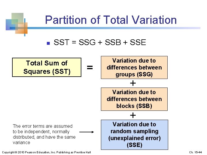
Partition of Total Variation n SST = SSG + SSB + SSE Total Sum of Squares (SST) = Variation due to differences between groups (SSG) + Variation due to differences between blocks (SSB) + The error terms are assumed to be independent, normally distributed, and have the same variance Copyright © 2010 Pearson Education, Inc. Publishing as Prentice Hall Variation due to random sampling (unexplained error) (SSE) Ch. 15 -44

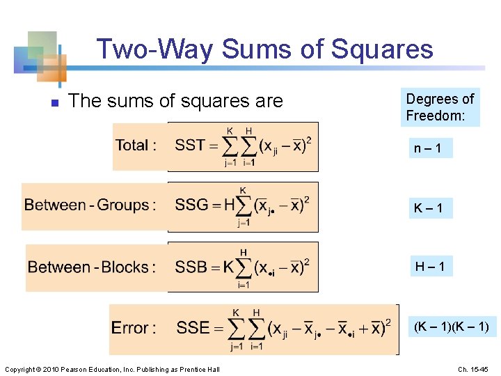
Two-Way Sums of Squares n The sums of squares are Degrees of Freedom: n

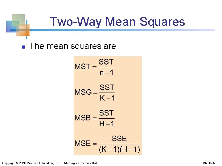
Two-Way Mean Squares n The mean squares are Copyright © 2010 Pearson Education, Inc.

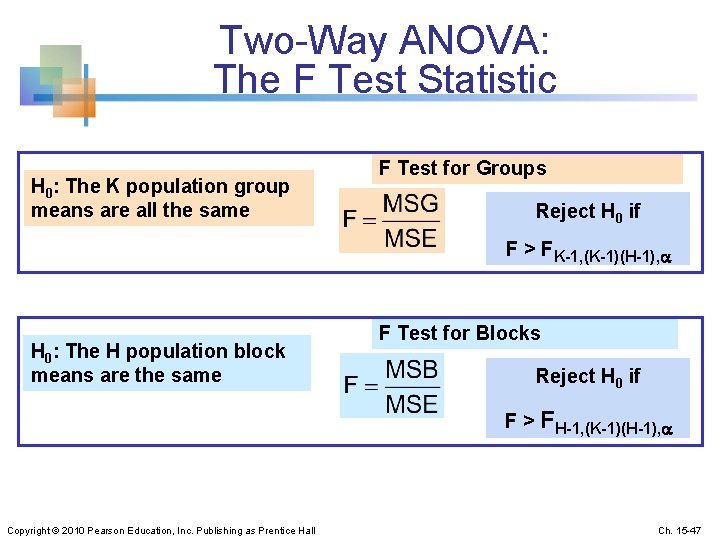
Two-Way ANOVA: The F Test Statistic H 0: The K population group means are all the same F Test for Groups Reject H 0 if F > FK-1, (K-1)(H-1), H 0: The H population block means are the same F Test for Blocks Reject H 0 if F > FH-1, (K-1)(H-1), Copyright © 2010 Pearson Education, Inc. Publishing as Prentice Hall Ch. 15 -47

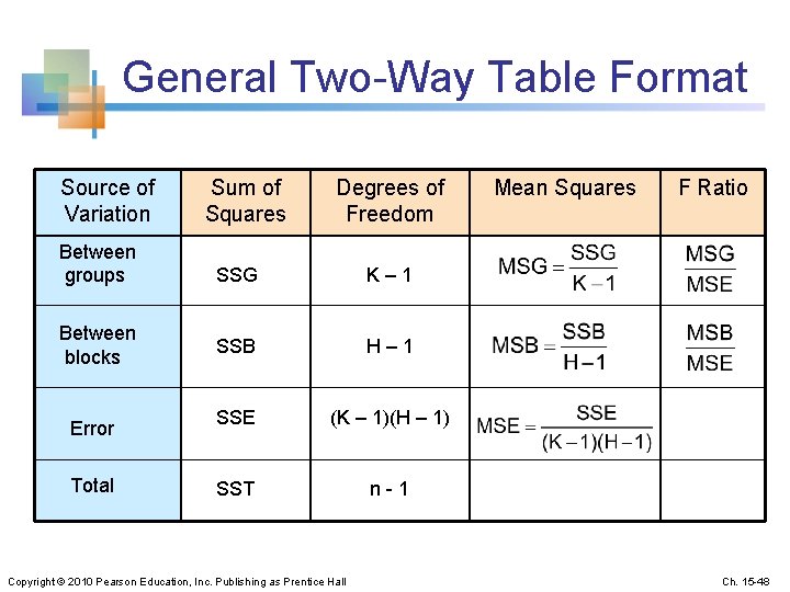
General Two-Way Table Format Source of Variation Between groups Between blocks Error Total Sum of Squares Degrees of Freedom SSG K – 1 SSB H – 1 SSE (K – 1)(H – 1) SST n - 1 Copyright © 2010 Pearson Education, Inc. Publishing as Prentice Hall Mean Squares F Ratio Ch. 15 -48

More than One Observation per Cell 15. 5 n n n A two-way design with more than one observation per cell allows one further source of variation The interaction between groups and blocks can also be identified Let n n K = number of groups H = number of blocks L = number of observations per cell n = KHL = total number of observations Copyright © 2010 Pearson Education, Inc. Publishing as Prentice Hall Ch. 15 -49

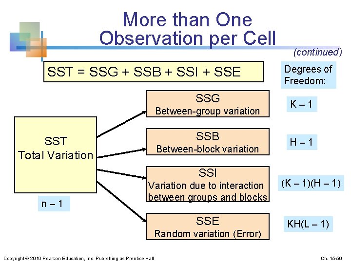
More than One Observation per Cell SST = SSG + SSB + SSI + SSE SSG Between-group variation SSB SST Total Variation Between-block variation SSI n – 1 (continued) Degrees of Freedom: K – 1 H – 1 Variation due to interaction between groups and blocks (K – 1)(H – 1) SSE KH(L – 1) Random variation (Error) Copyright © 2010 Pearson Education, Inc. Publishing as Prentice Hall Ch. 15 -50

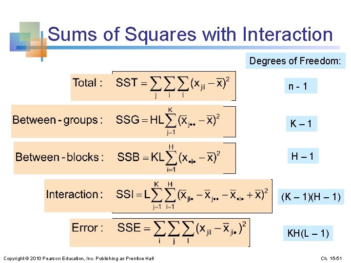
Sums of Squares with Interaction Degrees of Freedom: n - 1 K – 1

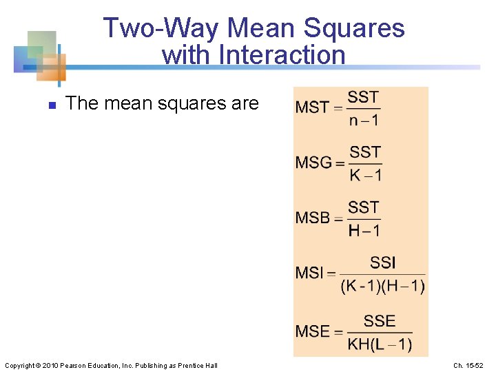
Two-Way Mean Squares with Interaction n The mean squares are Copyright © 2010 Pearson

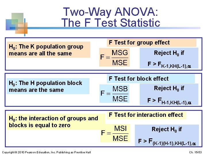
Two-Way ANOVA: The F Test Statistic H 0: The K population group means are all the same F Test for group effect Reject H 0 if F > FK-1, KH(L-1), H 0: The H population block means are the same F Test for block effect Reject H 0 if F > FH-1, KH(L-1), H 0: the interaction of groups and blocks is equal to zero F Test for interaction effect Reject H 0 if F > F(K-1)(H-1), KH(L-1), Copyright © 2010 Pearson Education, Inc. Publishing as Prentice Hall Ch. 15 -53

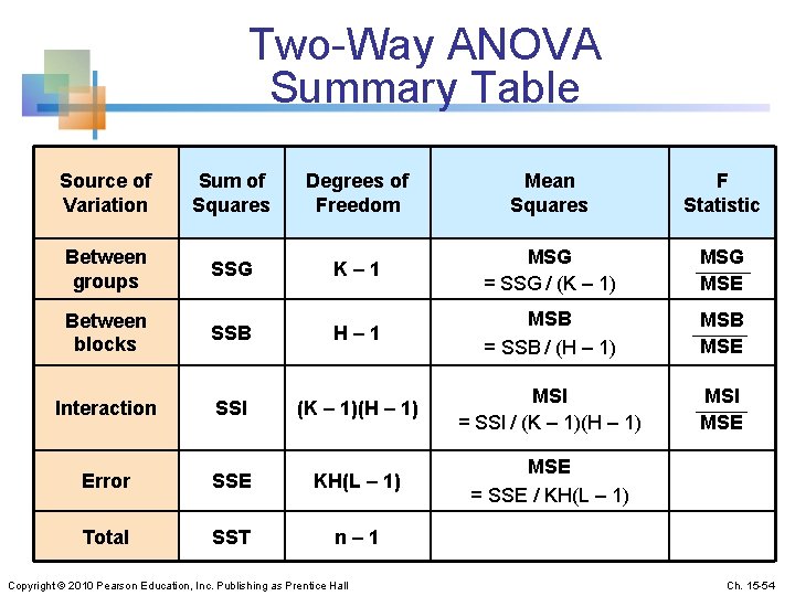
Two-Way ANOVA Summary Table Source of Variation Sum of Squares Degrees of Freedom Mean Squares F Statistic Between groups SSG K– 1 MSG = SSG / (K – 1) MSG MSE Between blocks SSB H– 1 MSB = SSB / (H – 1) MSB MSE Interaction SSI (K – 1)(H – 1) MSI = SSI / (K – 1)(H – 1) MSI MSE Error SSE KH(L – 1) MSE = SSE / KH(L – 1) Total SST n– 1 Copyright © 2010 Pearson Education, Inc. Publishing as Prentice Hall Ch. 15 -54

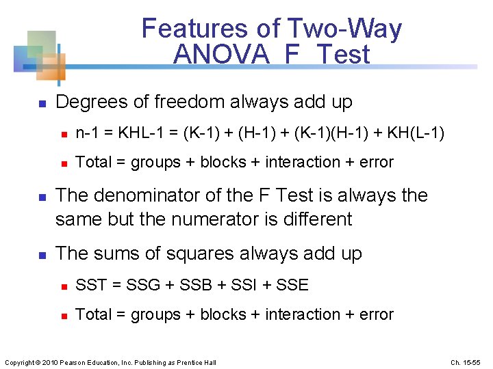
Features of Two-Way ANOVA F Test n n n Degrees of freedom always add up n n-1 = KHL-1 = (K-1) + (H-1) + (K-1)(H-1) + KH(L-1) n Total = groups + blocks + interaction + error The denominator of the F Test is always the same but the numerator is different The sums of squares always add up n SST = SSG + SSB + SSI + SSE n Total = groups + blocks + interaction + error Copyright © 2010 Pearson Education, Inc. Publishing as Prentice Hall Ch. 15 -55

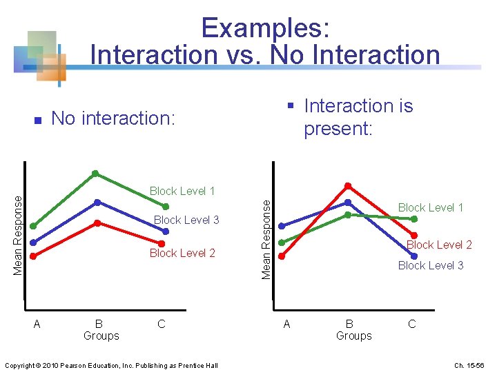
Examples: Interaction vs. No Interaction No interaction: Block Level 1 Block Level 3 Block Level 2 A B C Groups Copyright © 2010 Pearson Education, Inc. Publishing as Prentice Hall Mean Response n § Interaction is present: Block Level 1 Block Level 2 Block Level 3 A B C Groups Ch. 15 -56

Chapter Summary n Described one-way analysis of variance n n n The logic of Analysis of Variance assumptions F test for difference in K means Applied the Kruskal-Wallis test when the populations are not known to be normal Described two-way analysis of variance n n Examined effects of multiple factors Examined interaction between factors Copyright © 2010 Pearson Education, Inc. Publishing as Prentice Hall Ch. 15 -57