Statistics Biology Shellys Super Happy Fun Times February

Statistics & Biology Shelly’s Super Happy Fun Times February 7, 2012 Will Herrick

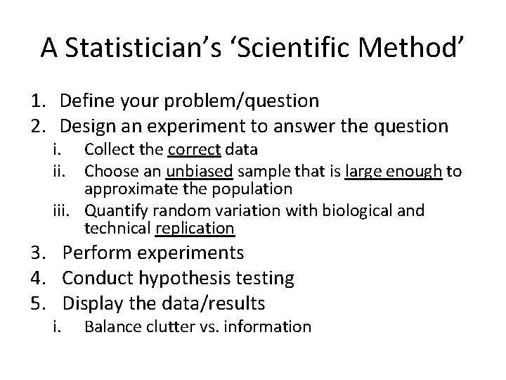
A Statistician’s ‘Scientific Method’ 1. Define your problem/question 2. Design an experiment to answer the question i. Collect the correct data ii. Choose an unbiased sample that is large enough to approximate the population iii. Quantify random variation with biological and technical replication 3. Perform experiments 4. Conduct hypothesis testing 5. Display the data/results i. Balance clutter vs. information

Important Terms • Categorical vs Quantitative Variables/Data • Random Variable • Mean: • Median • Percentiles • Variance: • Standard Deviation: • Range • Interquartile Range IQR = Q 3 – Q 1 • Outliers: Q 1 – 1. 5 x IQR > Outliers > Q 3 + 1. 5 x IQR

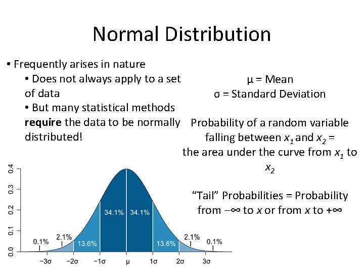
Normal Distribution • Frequently arises in nature • Does not always apply to a set μ = Mean of data σ = Standard Deviation • But many statistical methods require the data to be normally Probability of a random variable distributed! falling between x 1 and x 2 = the area under the curve from x 1 to x 2 “Tail” Probabilities = Probability from –∞ to x or from x to +∞

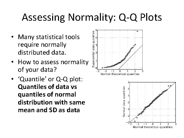
Assessing Normality: Q-Q Plots • Many statistical tools require normally distributed data. • How to assess normality of your data? • ‘Quantile’ or Q-Q plot: Quantiles of data vs quantiles of normal distribution with same mean and SD as data

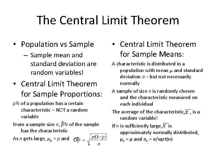
The Central Limit Theorem • Population vs Sample – Sample mean and standard deviation are random variables! • Central Limit Theorem for Sample Proportions: p% of a population has a certain characteristic – NOT a random variable From a sample size n, ^p% of the sample has the characteristic As n gets large, μp = p and • Central Limit Theorem for Sample Means: A characteristic is distributed in a population with mean μ and standard deviation σ – but not necessarily normally A sample of size n is randomly chosen and the characteristic measured on each individual The average of the characteristic, , is a random variable! If n is sufficiently large, is approximately normally distributed, μx = μ and σx = σ/sqrt(n)

Error Bars: Standard Deviation vs Standard Error • Standard Deviation: The variation of a characteristic within a population. – Independent of n! – More informative • Standard Error: AKA the ‘standard deviation of the mean, ’ this is how the sample mean varies with different samples. – Remember sample means are random variables subject to experimental error – It equals SD/sqrt(n)

Error Bars: Confidence Intervals • “ 95% Confidence Interval: ” the • When to Use: range of values that the Standard Deviation: When n is population mean could be very large and/or you wish to within with 95% confidence: emphasize the spread within the population. Standard Error: When comparing means between populations and have moderate n. • This is the 95% confidence Confidence Intervals: When interval for large n (> 40) comparing between • For smaller n or different %, populations; frequently used the equation is modified in medicine for ease of slightly. Versions for interpretation. population proportions exist Range: Almost never. too.

Design of Experiments: Statistical Models • Mathematical models • Ex: Suppose it’s known are deterministic, but that x (independent) statistical models are and y (dependent) have random. a linear relationship: • Given a set of data, fit it to a model so that • Here, the β’s are dependent variables can parameters and ε is an be predicted from error term of known independent variables. distribution. – But never exactly! • Find the parameters make predictions

Design of Experiments: Choosing Statistical Models • Quantitative vs Quantitative: Regression Model (curve fitting) • Categorical (dependent) vs Quantitative (independent): Logistic Regression, Multivariate Logistic Regression • Quantitative (dependent) vs Categorical (independent): ANOVA Model • Categorical vs Categorical: Contingency Tables

Design of Experiments: Sampling Problems • Bias: Systematic over • Adjust sampling or under-representation techniques to solve of a particular accuracy problems characteristic. • Increase the sample size • Accuracy: a measure of to improve precision bias. Unbiased samples are more accurate. • Precision: measure of variability in the measurements

Hypothesis Testing • Null Hypothesis, H 0: – A claim about the population parameter being measured – Formulated as an equality – The less exciting outcome i. e. “No difference between groups” • Alternative Hypothesis, Ha : – The opposite of the null hypothesis – What the scientist typically expects to be true – Formulated as <, > or ≠ relation

Hypothesis Testing: Example • Example: Comparing HASMC proliferation on collagen I and collagen III. • The null hypothesis: the proliferation on both collagens is the same. • The alternative hypothesis: the proliferation on collagens I and III is not the same. H 0 : μcollagen I = μcollagen III Ha : μcollagen I ≠ μcollagen III

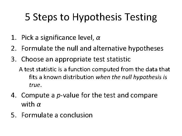
5 Steps to Hypothesis Testing 1. Pick a significance level, α 2. Formulate the null and alternative hypotheses 3. Choose an appropriate test statistic A test statistic is a function computed from the data that fits a known distribution when the null hypothesis is true. 4. Compute a p-value for the test and compare with α 5. Formulate a conclusion

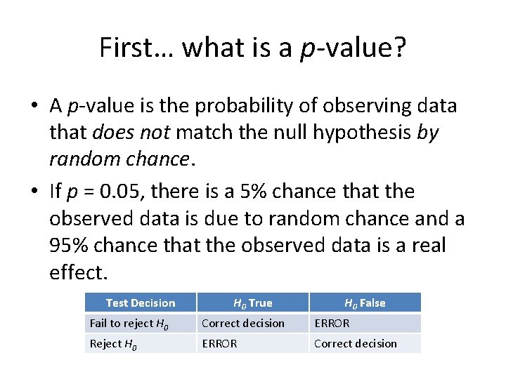
First… what is a p-value? • A p-value is the probability of observing data that does not match the null hypothesis by random chance. • If p = 0. 05, there is a 5% chance that the observed data is due to random chance and a 95% chance that the observed data is a real effect. Test Decision H 0 True H 0 False Fail to reject H 0 Correct decision ERROR Reject H 0 ERROR Correct decision

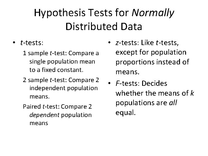
Hypothesis Tests for Normally Distributed Data • t-tests: 1 sample t-test: Compare a single population mean to a fixed constant. 2 sample t-test: Compare 2 independent population means. Paired t-test: Compare 2 dependent population means • z-tests: Like t-tests, except for population proportions instead of means. • F-tests: Decides whether the means of k populations are all equal.

Non-Parametric Tests for Abnormally Distributed Data • Wilcoxon-Mann-Whitney Rank Sum Test: Comparable to the 2 -sample t-test. • Non-parametric tests are more versatile, but less powerful. • Still have assumptions to satisfy!

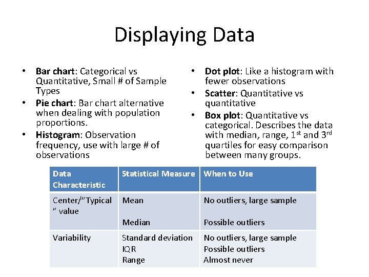
Displaying Data • Bar chart: Categorical vs Quantitative, Small # of Sample Types • Pie chart: Bar chart alternative when dealing with population proportions. • Histogram: Observation frequency, use with large # of observations • Dot plot: Like a histogram with fewer observations • Scatter: Quantitative vs quantitative • Box plot: Quantitative vs categorical. Describes the data with median, range, 1 st and 3 rd quartiles for easy comparison between many groups. Data Characteristic Statistical Measure When to Use Center/”Typical ” value Mean No outliers, large sample Median Possible outliers Variability Standard deviation IQR Range No outliers, large sample Possible outliers Almost never

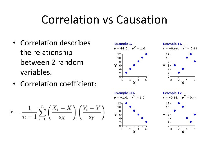
Correlation vs Causation • Correlation describes the relationship between 2 random variables. • Correlation coefficient:

Biological vs Technical Replicates • All the cells in 1 flask are • To increase n, the considered 1 biological number of samples, we source must repeat experiments with • Therefore, replicate different flasks of cells! wells of cells seeded for an experiment are • It is not appropriate to technical replicates. use error bars if you have not repeated the • They only measure experiment with variability due to biological replicates. experimental error!

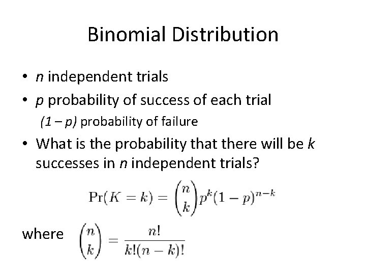
Binomial Distribution • n independent trials • p probability of success of each trial (1 – p) probability of failure • What is the probability that there will be k successes in n independent trials? where