Statistics 349 302 Statistics 846 302 Analysis of

Statistics 349. 3(02) Statistics 846. 3(02) Analysis of Time Series

Course Information 1. Instructor: • • • W. H. Laverty 235 Mc. Lean Hall Tel: 966 -6096 Email: laverty@math. usask. ca 2. Class Times • MWF 12: 30 -1: 20 pm Thorv 110 3. Mark break-up • • Final Exam – 60% Term Tests and Assignments – 40%

Course Outline 1. Introduction and Review of Probability Theory – Probability distributions, Expectation, Variance, correlation – Sampling distributions – Estimation Theory – Hypothesis Testing

Course Outline -continued 2. Fundamental concepts in Time Series Analysis – Stationarity – Autocovariance function, autocorrelation and partial autocorrelation function 3. Models for Stationary Time series – Autoregressive (AR), Moving average (MA), mixed Autoregressive-Moving average (ARMA) models 4. Models for Non-stationary Time series – ARIMA (Integrated Autoregressive-Moving average models)

Course Outline -continued 5. 6. 7. 8. Forecasting ARIMA Processes Model Identification and Estimation Models for seasonal Time series Spectral Analysis of Time series

Course Outline -continued 9. State-Space modeling of time series, Hidden Markov Model (HMM) – Kalman filtering 10. Multivariate (Multi-channel) time series analysis 11. Linear filtering

Comments • The Text Book (non assigned) • I will present the material in power point slides that will be available on my web site. • Hopefully this makes purchasing the text book optional. It is useful for students to purchase text books and build up a library.

References 1. Introduction to Statistical Time Series (2 nd Ed. ) – Wayne A. Fuller 2. Applied Statistical Time Series Analysis, for managerial forecasting, C R. Nelson 3. Time Series Analysis - Forecasting and Control, Box and Jenkins 4. Applied Statistical Time Series Analysis, Robert H. Shumway.

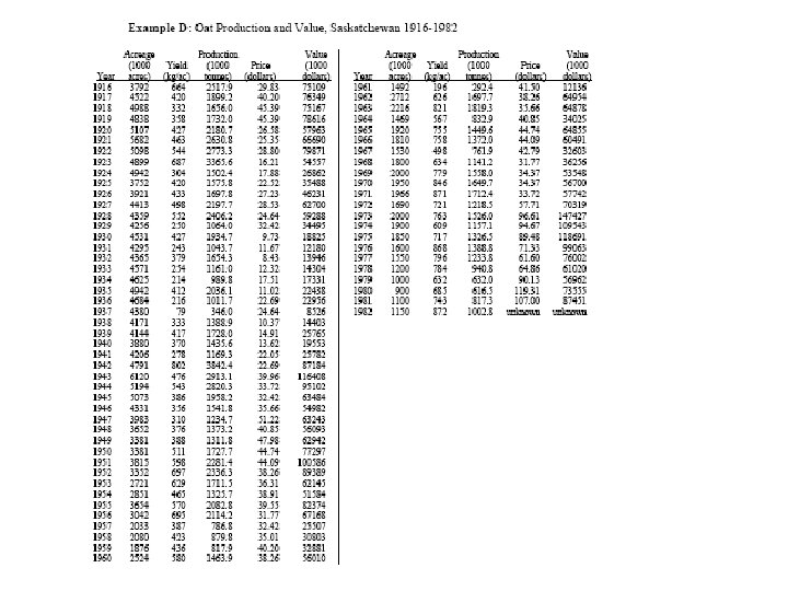
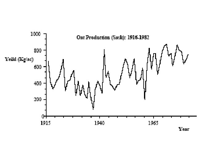
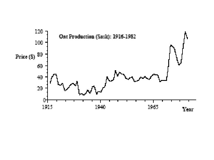
Some examples of Time series data

IBM Stock Price (closing)

Time Sequence plot

Concentration of residue after production of a chemical

Time Sequence plot

Yearly sunspot activity (1770 -1869)

Time Sequence plot

Time Sequence Plots

Example Measuring brain activity in an insect as an object is approaching. Time t = 0 is at the point of impact.

Simulation To aid in the understanding of time series it is useful to simulate data

Generating observations from a distribution

Generating a random number from a distribution Let 1. f(x) denote the density function 2. F(x) denote the cumulative distribution function = P[X ≤ x] 3. F-1(x) denote the inverse cumulative distribution function

f(x) F(x) denote the cumulative distribution function F(x) x

f(x) u F(x) denote the cumulative distribution function F-1(u) If u is chosen at random from 0 to 1 then x = F-1(u) is chosen at random from the density f(x). In EXCEL the following function generates a random observation from a normal distribution. = NORMINV(RAND(), mean, standard deviation)

Example Random walk A random walk is a sequence of random variables {xt} satisfying: x t = x t – 1 + ut where {ut} is a sequence of independent random variables having mean 0, standard deviation s. (usually normally distributed) The excel functions 1. NORMINV(prob, mean, standard deviation) computes F-1(prob) for the normal distribution. 2. RAND() computes and random number from the Uniform distribution from 0 to 1. 3. NORMINV(RAND(), mean, standard deviation) computes and random number from the Normal distribution with a given mean and standard deviation.