Statistics 262 Intermediate Biostatistics May 11 2004 Cox

Statistics 262: Intermediate Biostatistics May 11, 2004: Cox Regression II: tied data, PH assumption, time-dependent covariates Jonathan Taylor and Kristin Cobb Satistics 262 1

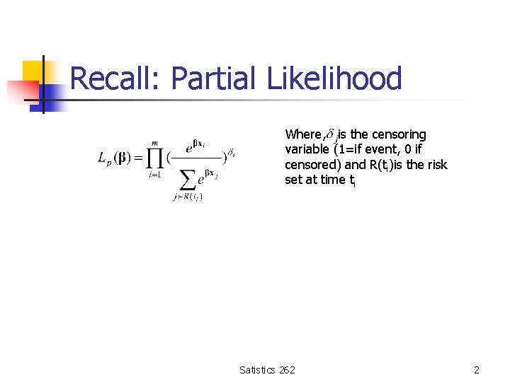
Recall: Partial Likelihood Where, is the censoring variable (1=if event, 0 if censored) and R(ti)is the risk set at time ti Satistics 262 2

Ties n n The PL assumed no tied values among the observed survival times Not often the case with real data Satistics 262 3

Ties n n Exact method (time is continuous; ties are a result of imprecise measurement of time) Breslow approximation (SAS default) Efron approximation Discrete method (treats time as discrete; ties are real) In SAS: option on the model statement: ties=exact/efron/breslow/discrete Satistics 262 4

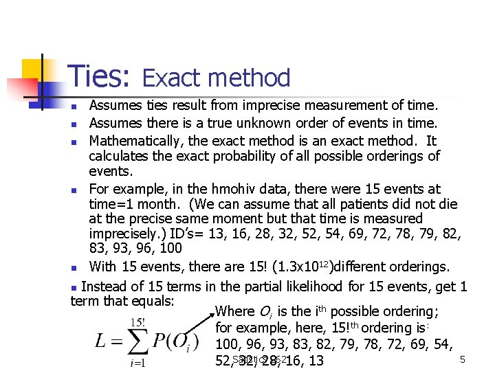
Ties: Exact method Assumes ties result from imprecise measurement of time. n Assumes there is a true unknown order of events in time. n Mathematically, the exact method is an exact method. It calculates the exact probability of all possible orderings of events. n For example, in the hmohiv data, there were 15 events at time=1 month. (We can assume that all patients did not die at the precise same moment but that time is measured imprecisely. ) ID’s= 13, 16, 28, 32, 54, 69, 72, 78, 79, 82, 83, 96, 100 n With 15 events, there are 15! (1. 3 x 10 12)different orderings. n Instead of 15 terms in the partial likelihood for 15 events, get 1 term that equals: Where Oi is the ith possible ordering; for example, here, 15!th ordering is: 100, 96, 93, 82, 79, 78, 72, 69, 54, 26216, 13 5 52, Satistics 32, 28, n

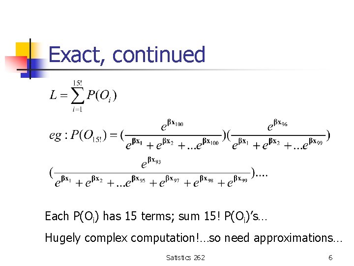
Exact, continued Each P(Oi) has 15 terms; sum 15! P(Oi)’s… Hugely complex computation!…so need approximations… Satistics 262 6

Breslow and Efron methods Breslow (1974) n Efron (1977) n Both are approximations to the exact method. both have much faster calculation times Breslow is SAS default. Breslow does not do well when the number of ties at a particular time point is a large proportion of the number of cases at risk. Prefer Efron to Breslow We’ll see how to implement in SAS today and Satistics 262 7 compare methods. n

Discrete method Assumes time is truly discrete. n When would time be discrete? When events are only periodic, such as: --Winning an Olympic medal (can only happen every 4 years) --Missing this class (can only happen on Tuesdays at 10 am) --Voting for President (can only happen every 4 years) n Satistics 262 8

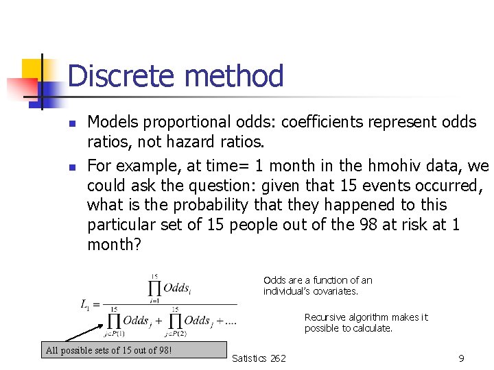
Discrete method n n Models proportional odds: coefficients represent odds ratios, not hazard ratios. For example, at time= 1 month in the hmohiv data, we could ask the question: given that 15 events occurred, what is the probability that they happened to this particular set of 15 people out of the 98 at risk at 1 month? Odds are a function of an individual’s covariates. Recursive algorithm makes it possible to calculate. All possible sets of 15 out of 98! Satistics 262 9

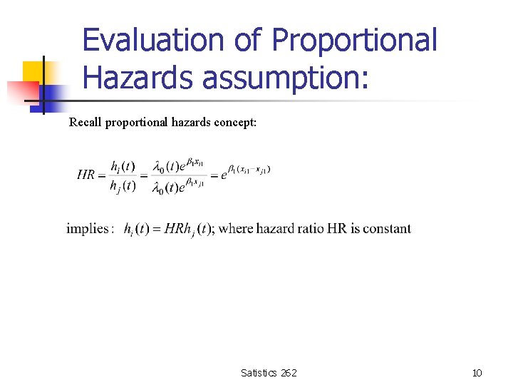
Evaluation of Proportional Hazards assumption: Recall proportional hazards concept: Satistics 262 10

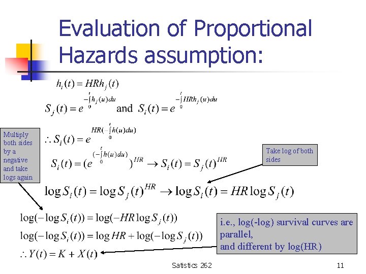
Evaluation of Proportional Hazards assumption: Multiply both sides by a negative and take logs again Take log of both sides i. e. , log(-log) survival curves are parallel, and different by log(HR) Satistics 262 11

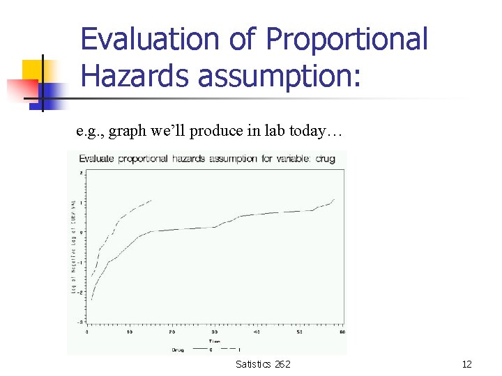
Evaluation of Proportional Hazards assumption: e. g. , graph we’ll produce in lab today… Satistics 262 12

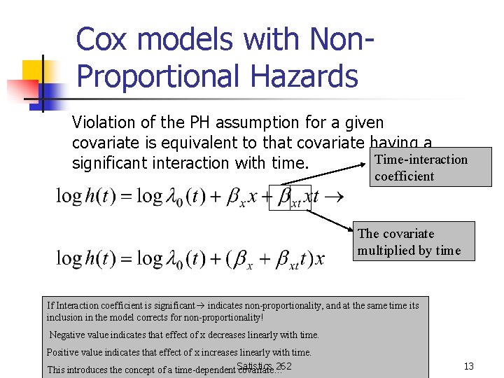
Cox models with Non. Proportional Hazards Violation of the PH assumption for a given covariate is equivalent to that covariate having a Time-interaction significant interaction with time. coefficient The covariate multiplied by time If Interaction coefficient is significant indicates non-proportionality, and at the same time its inclusion in the model corrects for non-proportionality! Negative value indicates that effect of x decreases linearly with time. Positive value indicates that effect of x increases linearly with time. 262 This introduces the concept of a time-dependent Satistics covariate… 13

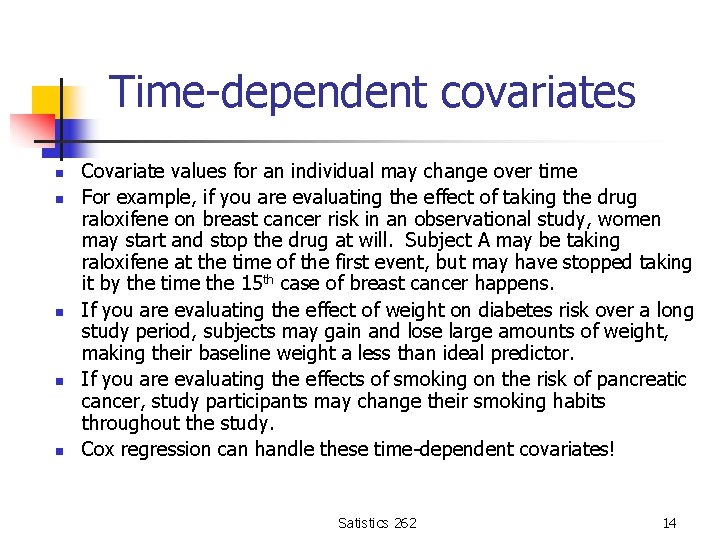
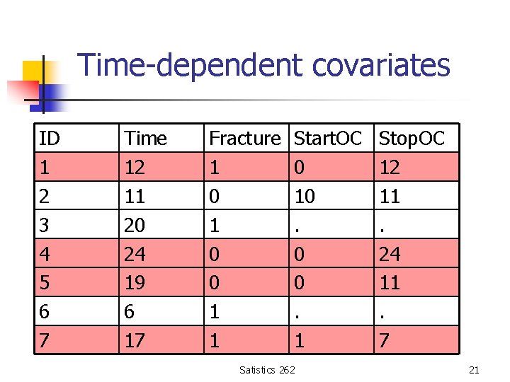
Time-dependent covariates n n n Covariate values for an individual may change over time For example, if you are evaluating the effect of taking the drug raloxifene on breast cancer risk in an observational study, women may start and stop the drug at will. Subject A may be taking raloxifene at the time of the first event, but may have stopped taking it by the time the 15 th case of breast cancer happens. If you are evaluating the effect of weight on diabetes risk over a long study period, subjects may gain and lose large amounts of weight, making their baseline weight a less than ideal predictor. If you are evaluating the effects of smoking on the risk of pancreatic cancer, study participants may change their smoking habits throughout the study. Cox regression can handle these time-dependent covariates! Satistics 262 14

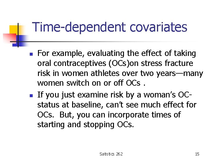
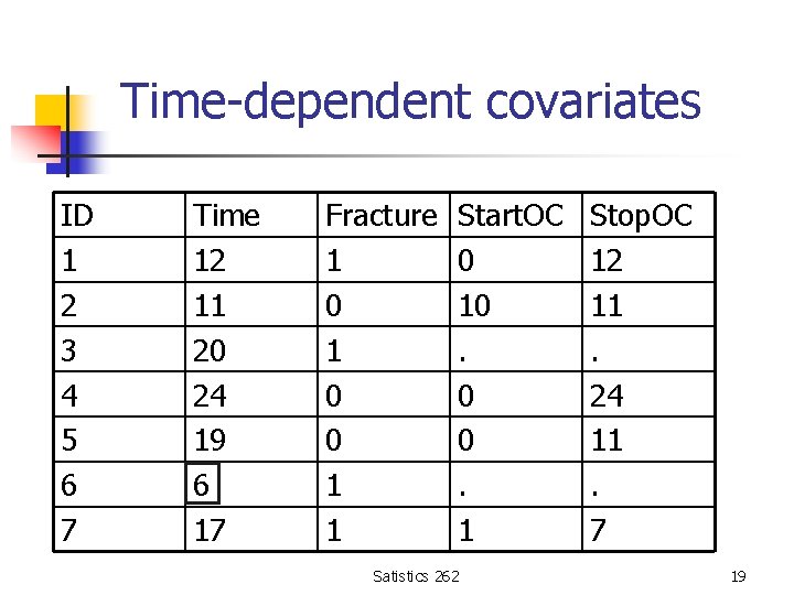
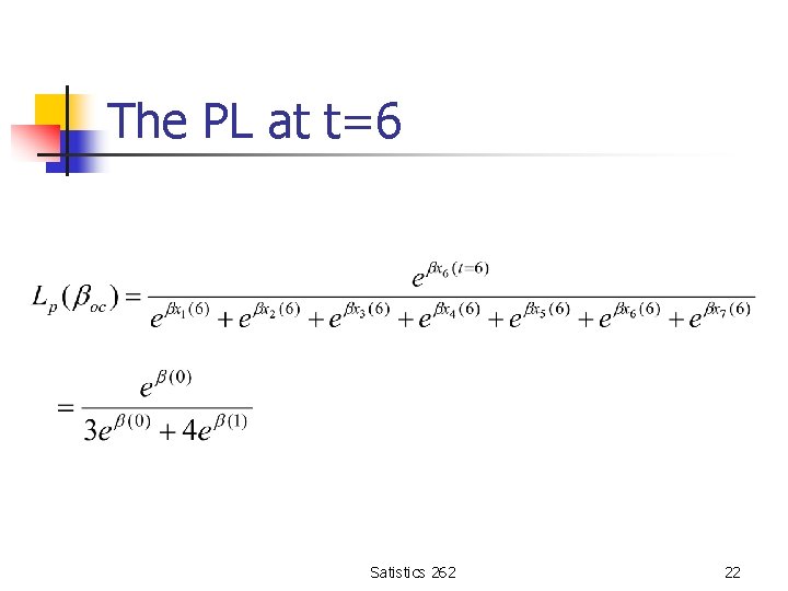
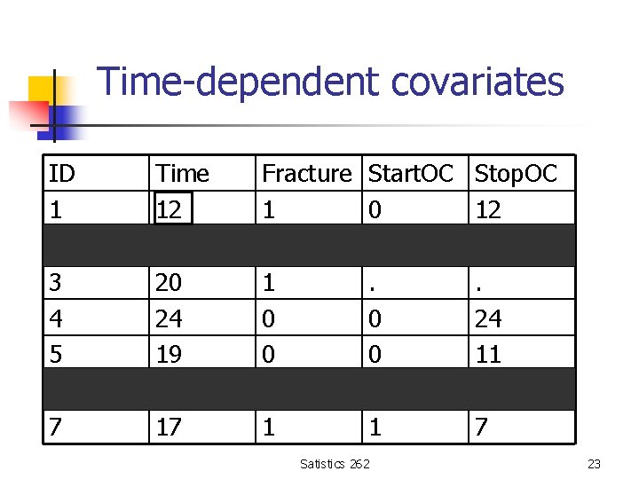
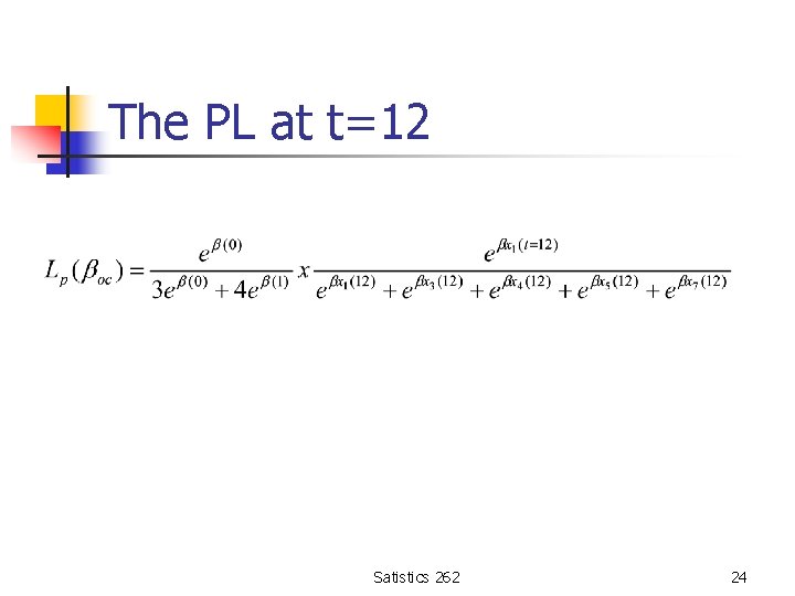
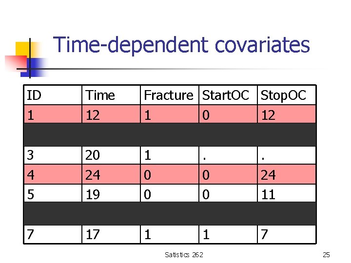
Time-dependent covariates n n For example, evaluating the effect of taking oral contraceptives (OCs)on stress fracture risk in women athletes over two years—many women switch on or off OCs. If you just examine risk by a woman’s OCstatus at baseline, can’t see much effect for OCs. But, you can incorporate times of starting and stopping OCs. Satistics 262 15

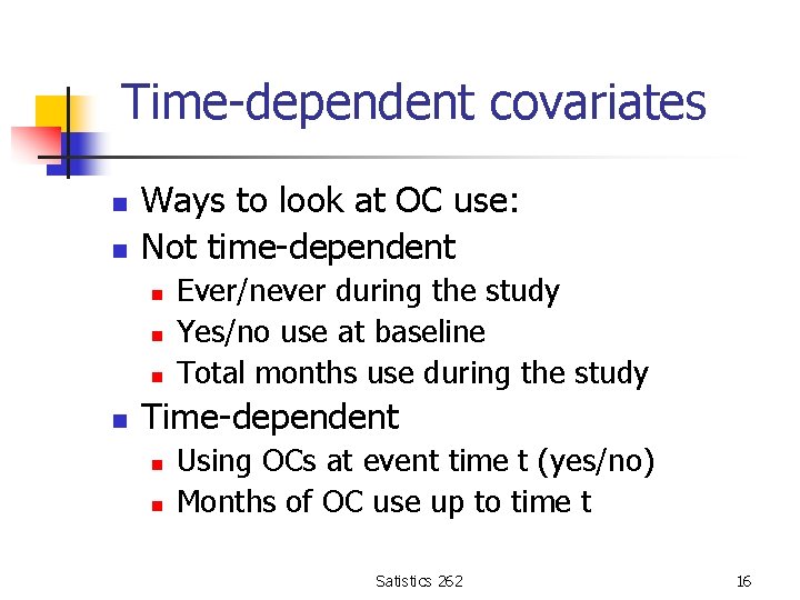
Time-dependent covariates n n Ways to look at OC use: Not time-dependent n n Ever/never during the study Yes/no use at baseline Total months use during the study Time-dependent n n Using OCs at event time t (yes/no) Months of OC use up to time t Satistics 262 16

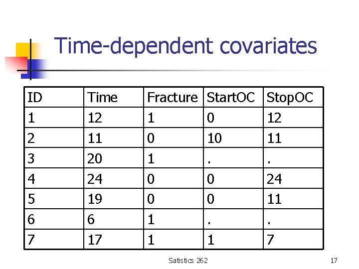
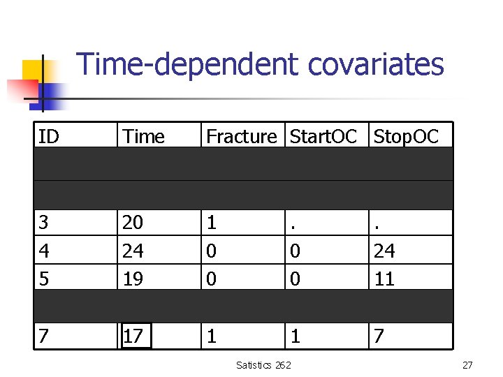
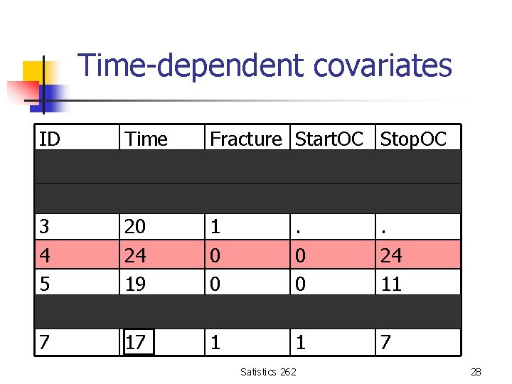
Time-dependent covariates ID 1 2 3 4 5 6 7 Time 12 11 20 24 19 6 17 Fracture 1 0 0 1 1 Start. OC 0 10. 0 0. 1 Satistics 262 Stop. OC 12 11. 24 11. 7 17

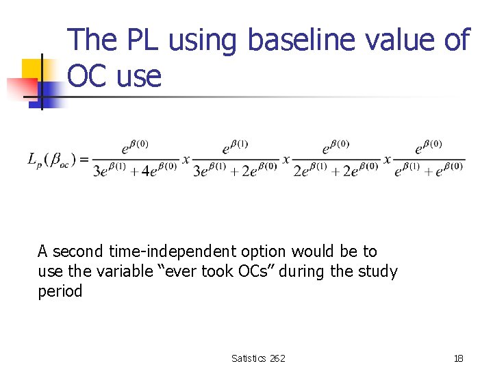
The PL using baseline value of OC use A second time-independent option would be to use the variable “ever took OCs” during the study period Satistics 262 18

Time-dependent covariates ID 1 2 3 4 5 6 7 Time 12 11 20 24 19 6 17 Fracture 1 0 0 1 1 Start. OC 0 10. 0 0. 1 Satistics 262 Stop. OC 12 11. 24 11. 7 19

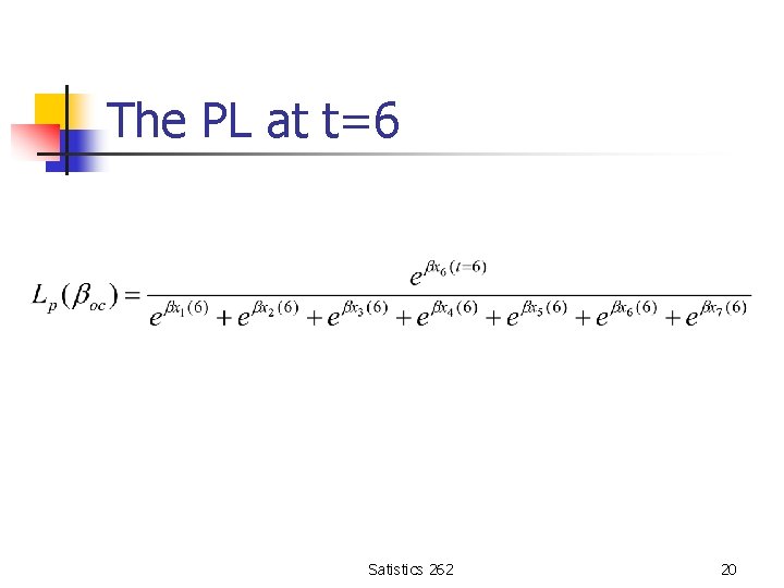
The PL at t=6 Satistics 262 20

Time-dependent covariates ID 1 2 3 4 5 6 7 Time 12 11 20 24 19 6 17 Fracture 1 0 0 1 1 Start. OC 0 10. 0 0. 1 Satistics 262 Stop. OC 12 11. 24 11. 7 21

The PL at t=6 Satistics 262 22

Time-dependent covariates ID 1 2 3 4 5 6 7 Time 12 11 20 24 19 6 17 Fracture 1 0 0 1 1 Start. OC 0 10. 0 0. 1 Satistics 262 Stop. OC 12 11. 24 11. 7 23

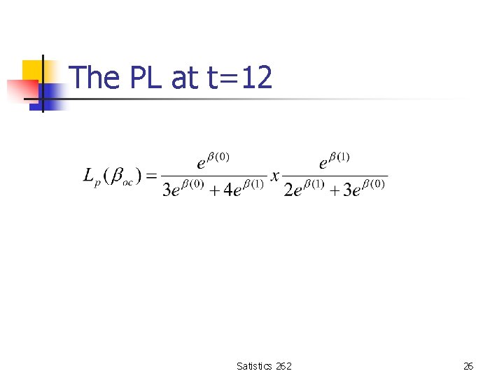
The PL at t=12 Satistics 262 24

Time-dependent covariates ID 1 2 3 4 5 6 7 Time 12 11 20 24 19 6 17 Fracture 1 0 0 1 1 Start. OC 0 10. 0 0. 1 Satistics 262 Stop. OC 12 11. 24 11. 7 25

The PL at t=12 Satistics 262 26

Time-dependent covariates ID 1 2 3 4 5 6 7 Time 12 11 20 24 19 6 17 Fracture 1 0 0 1 1 Start. OC 0 10. 0 0. 1 Satistics 262 Stop. OC 12 11. 24 11. 7 27

Time-dependent covariates ID 1 2 3 4 5 6 7 Time 12 11 20 24 19 6 17 Fracture 1 0 0 1 1 Start. OC 0 10. 0 0. 1 Satistics 262 Stop. OC 12 11. 24 11. 7 28

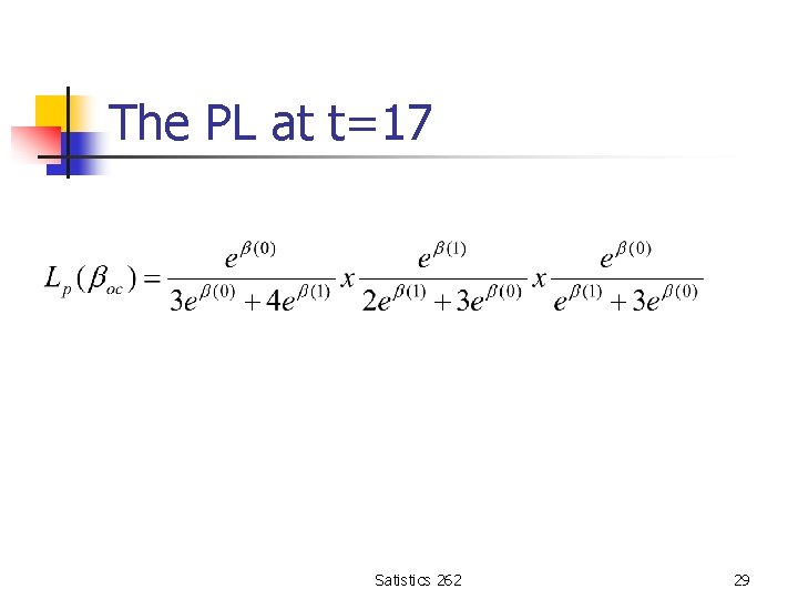
The PL at t=17 Satistics 262 29

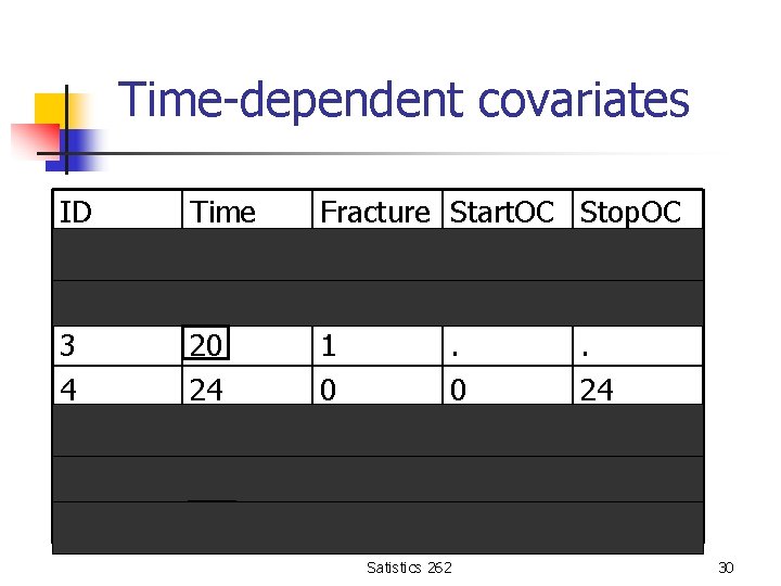
Time-dependent covariates ID 1 2 3 4 5 6 7 Time 12 11 20 24 19 6 17 Fracture 1 0 0 1 1 Start. OC 0 10. 0 0. 1 Satistics 262 Stop. OC 12 11. 24 11. 7 30

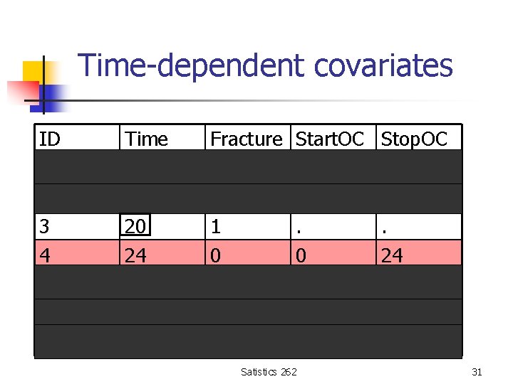
Time-dependent covariates ID 1 2 3 4 5 6 7 Time 12 11 20 24 19 6 17 Fracture 1 0 0 1 1 Start. OC 0 10. 0 0. 1 Satistics 262 Stop. OC 12 11. 24 11. 7 31

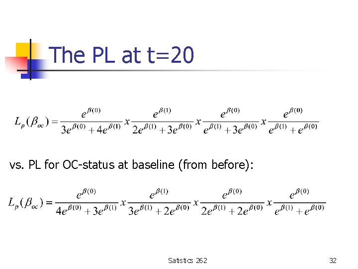
The PL at t=20 vs. PL for OC-status at baseline (from before): Satistics 262 32

Next week: Cox regression III n n n Diagnostics and influence statistics Sample size calculations Repeated events Satistics 262 33