Statistics 202 Statistical Aspects of Data Mining Professor

Statistics 202: Statistical Aspects of Data Mining Professor David Mease Tuesday, Thursday 9: 00 -10: 15 AM Terman 156 Lecture 7 = Finish chapter 3 and start chapter 6 Agenda: 1) Reminder about midterm exam (July 26) 2) Assign Chapter 6 homework (due 9 AM Tues) 3) Lecture over rest of Chapter 3 (section 3. 2) 4) Begin lecturing over Chapter 6 (section 6. 1) 1

Announcement – Midterm Exam: The midterm exam will be Thursday, July 26 The best thing will be to take it in the classroom (9: 0010: 15 AM in Terman 156) For remote students who absolutely can not come to the classroom that day please email me to confirm arrangements with SCPD You are allowed one 8. 5 x 11 inch sheet (front and back) for notes No books or computers are allowed, but please bring a hand held calculator The exam will cover the material that we covered in class from Chapters 1, 2, 3 and 6 2

Homework Assignment: Chapter 3 Homework Part 2 and Chapter 6 Homework is due 9 AM Tuesday 7/24 Either email to me (dmease@stanford. edu), bring it to class, or put it under my office door. SCPD students may use email or fax or mail. The assignment is posted at http: //www. stats 202. com/homework. html Important: If using email, please submit only a single file (word or pdf) with your name and chapters in the file name. Also, include your name on the first page. 3

Introduction to Data Mining by Tan, Steinbach, Kumar Chapter 3: Exploring Data 4

Exploring Data l. We can explore data visually (using tables or graphs) or numerically (using summary statistics) l. Section 3. 2 deals with summary statistics l. Section 3. 3 deals with visualization l. We will begin with visualization l. Note that many of the techniques you use to explore data are also useful for presenting data 5

Final Touches Many times plots are difficult to read or unattractive because people do not take the time to learn how to adjust default values for font size, font type, color schemes, margin size, plotting characters, etc. l l In R, the function par() controls a lot of these Also in R, the command expression() can produce subscripts and Greek letters in the text -example: xlab=expression(alpha[1]) l In Excel, it is often difficult to get exactly what you want, but you can usually improve upon the default values l 6

Exploring Data l. We can explore data visually (using tables or graphs) or numerically (using summary statistics) l. Section 3. 2 deals with summary statistics l. Section 3. 3 deals with visualization l. We will begin with visualization l. Note that many of the techniques you use to explore data are also useful for presenting data 7

Summary Statistics (Section 3. 2, Page 98): You should be familiar with the following elementary summary statistics: l -Measures of Location: Percentiles (page 100) Mean (page 101) Median (page 101) -Measures of Spread: Range (page 102) Variance (page 103) Standard Deviation (page 103) Interquartile Range (page 103) -Measures of Association: Covariance (page 104) Correlation (page 104) 8

Measures of Location l Terminology: the “mean” is the average l Terminology: the “median” is the 50 th percentile Your book classifies only the mean and median as measures of location but not percentiles l More commonly, all three are thought of as measures of location and the mean and median are more specifically measures of center l Terminology: the 1 st, 2 nd and 3 rd quartiles are the 25 th, 50 th and 75 th percentiles respectively l 9

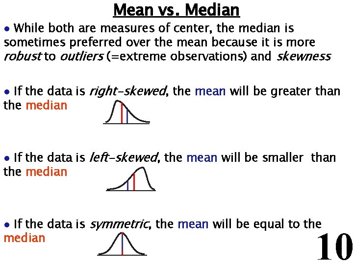
Mean vs. Median While both are measures of center, the median is sometimes preferred over the mean because it is more robust to outliers (=extreme observations) and skewness l If the data is right-skewed, the mean will be greater than the median l If the data is left-skewed, the mean will be smaller than the median l If the data is symmetric, the mean will be equal to the median l 10

11

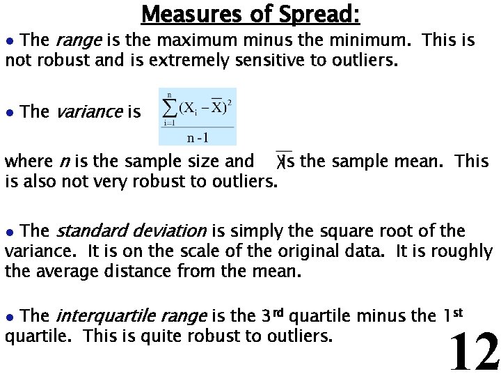
Measures of Spread: The range is the maximum minus the minimum. This is not robust and is extremely sensitive to outliers. l l The variance is where n is the sample size and is the sample mean. This is also not very robust to outliers. The standard deviation is simply the square root of the variance. It is on the scale of the original data. It is roughly the average distance from the mean. l The interquartile range is the 3 rd quartile minus the 1 st quartile. This is quite robust to outliers. l 12

In class exercise #22: Compute the standard deviation for this data by hand: 2 10 22 43 18 Confirm that R and Excel give the same values. 13

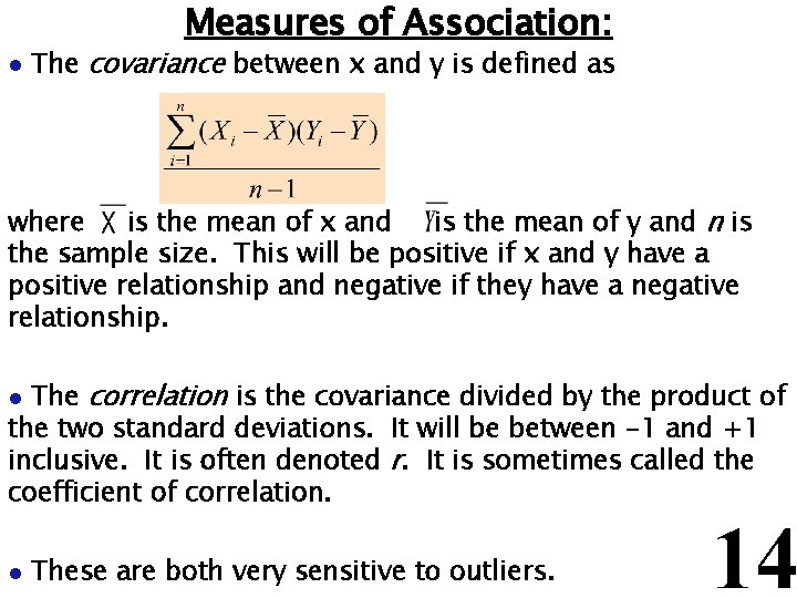
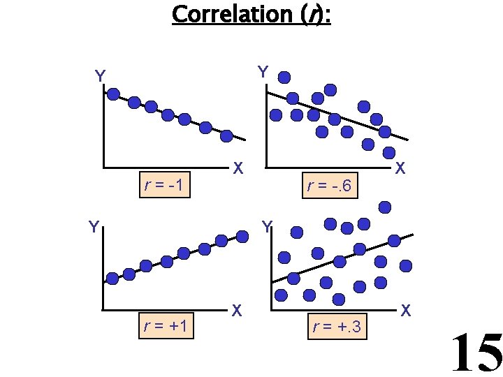
Measures of Association: l The covariance between x and y is defined as where is the mean of x and is the mean of y and n is the sample size. This will be positive if x and y have a positive relationship and negative if they have a negative relationship. The correlation is the covariance divided by the product of the two standard deviations. It will be between -1 and +1 inclusive. It is often denoted r. It is sometimes called the coefficient of correlation. l l These are both very sensitive to outliers. 14

Correlation (r): Y Y r = -1 X Y r = -. 6 X Y r = +1 X r = +. 3 X 15

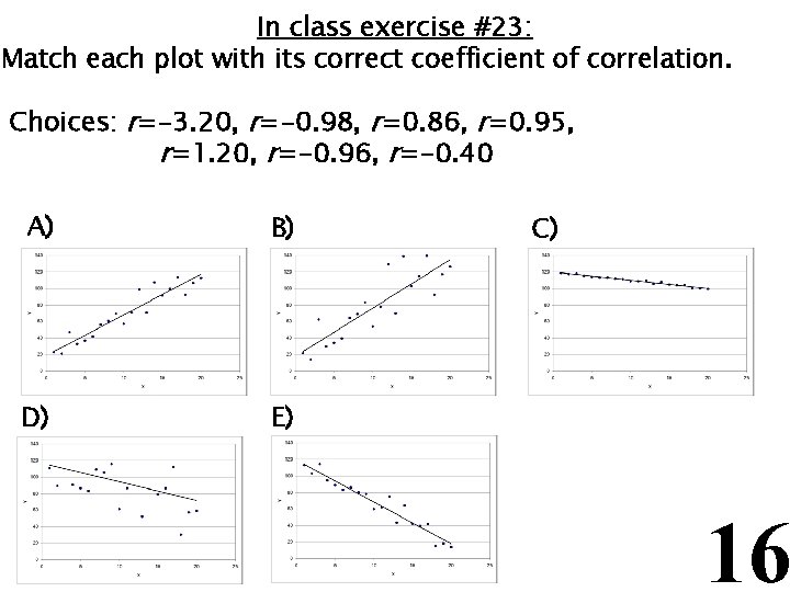
In class exercise #23: Match each plot with its correct coefficient of correlation. Choices: r=-3. 20, r=-0. 98, r=0. 86, r=0. 95, r=1. 20, r=-0. 96, r=-0. 40 A) B) D) E) C) 16

In class exercise #24: Make two vectors of length 1, 000 in R using runif(1000000) and compute the coefficient of correlation using cor(). Does the resulting value surprise you? 17

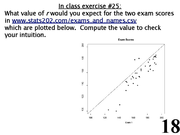
In class exercise #25: What value of r would you expect for the two exam scores in www. stats 202. com/exams_and_names. csv which are plotted below. Compute the value to check your intuition. 18

Introduction to Data Mining by Tan, Steinbach, Kumar Chapter 6: Association Analysis 19

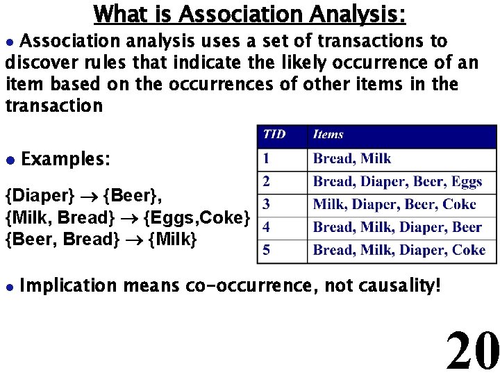
What is Association Analysis: Association analysis uses a set of transactions to discover rules that indicate the likely occurrence of an item based on the occurrences of other items in the transaction l l Examples: {Diaper} {Beer}, {Milk, Bread} {Eggs, Coke} {Beer, Bread} {Milk} l Implication means co-occurrence, not causality! 20

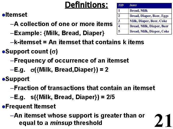
Definitions: l. Itemset –A collection of one or more items –Example: {Milk, Bread, Diaper} –k-itemset = An itemset that contains k items l. Support count ( ) –Frequency of occurrence of an itemset –E. g. ({Milk, Bread, Diaper}) = 2 l. Support –Fraction of transactions that contain an itemset –E. g. s({Milk, Bread, Diaper}) = 2/5 l. Frequent Itemset –An itemset whose support is greater than or equal to a minsup threshold 21

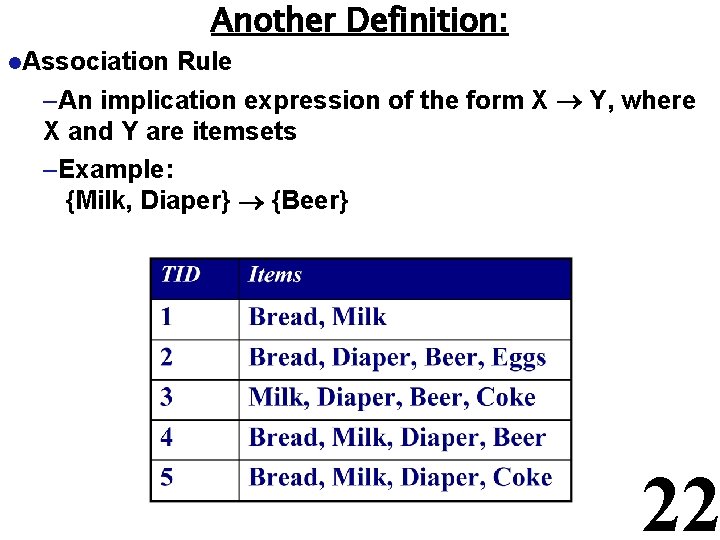
Another Definition: l. Association Rule –An implication expression of the form X Y, where X and Y are itemsets –Example: {Milk, Diaper} {Beer} 22

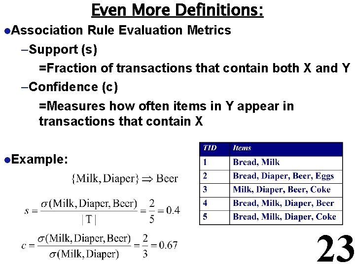
Even More Definitions: l. Association Rule Evaluation Metrics –Support (s) =Fraction of transactions that contain both X and Y –Confidence (c) =Measures how often items in Y appear in transactions that contain X l. Example: 23

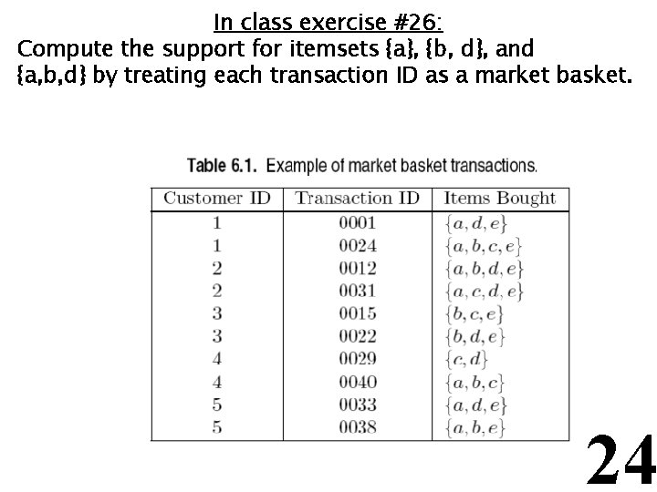
In class exercise #26: Compute the support for itemsets {a}, {b, d}, and {a, b, d} by treating each transaction ID as a market basket. 24

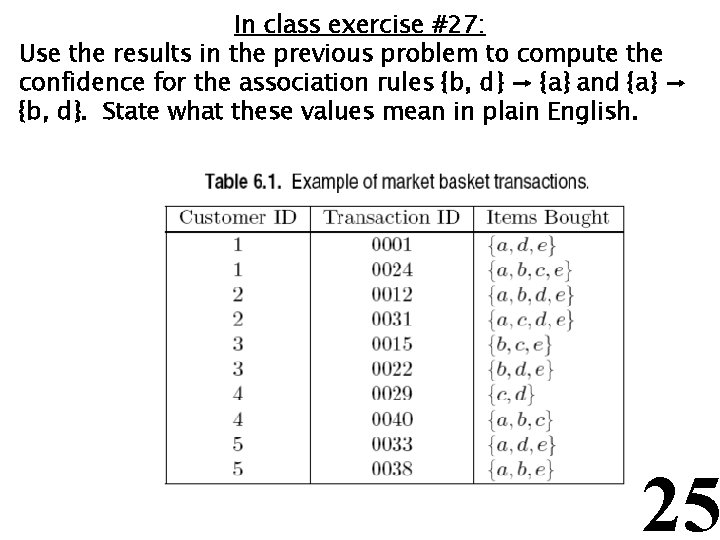
In class exercise #27: Use the results in the previous problem to compute the confidence for the association rules {b, d} → {a} and {a} → {b, d}. State what these values mean in plain English. 25

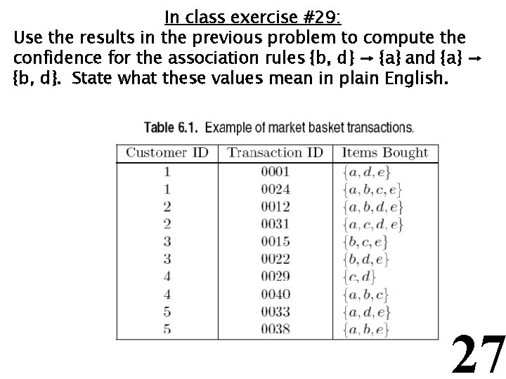
In class exercise #28: Compute the support for itemsets {a}, {b, d}, and {a, b, d} by treating each customer ID as a market basket. 26

In class exercise #29: Use the results in the previous problem to compute the confidence for the association rules {b, d} → {a} and {a} → {b, d}. State what these values mean in plain English. 27

In class exercise #30: The data www. stats 202. com/more_stats 202_logs. txt contains access logs from May 7, 2007 to July 1, 2007. Treating each row as a "market basket" find the support and confidence for the rule Mozilla/5. 0 (compatible; Yahoo! Slurp; http: //help. yahoo. com/help/us/ysearch/slurp)→ 74. 6. 19. 105 28

An Association Rule Mining Task: l Given a set of transactions T, find all rules having both - support ≥ minsup threshold - confidence ≥ minconf threshold l Brute-force approach: - List all possible association rules - Compute the support and confidence for each rule - Prune rules that fail the minsup and minconf thresholds - Problem: this is computationally prohibitive! 29

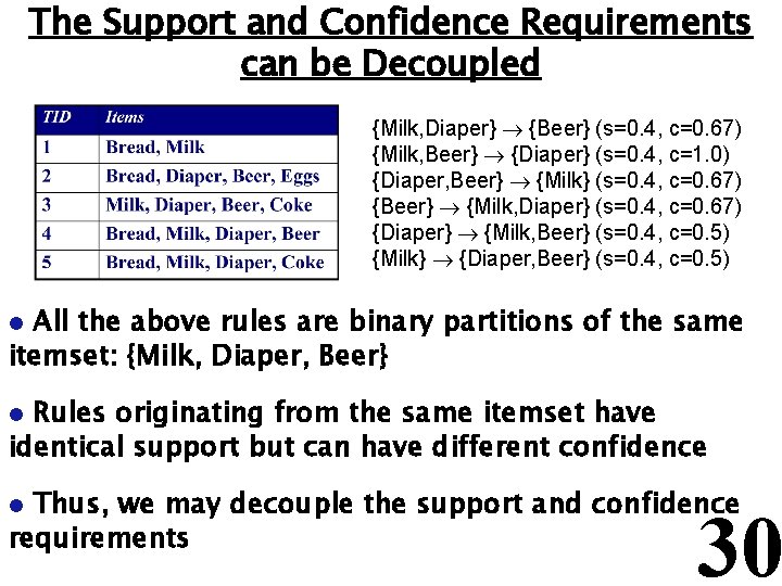
The Support and Confidence Requirements can be Decoupled {Milk, Diaper} {Beer} (s=0. 4, c=0. 67) {Milk, Beer} {Diaper} (s=0. 4, c=1. 0) {Diaper, Beer} {Milk} (s=0. 4, c=0. 67) {Beer} {Milk, Diaper} (s=0. 4, c=0. 67) {Diaper} {Milk, Beer} (s=0. 4, c=0. 5) {Milk} {Diaper, Beer} (s=0. 4, c=0. 5) All the above rules are binary partitions of the same itemset: {Milk, Diaper, Beer} l Rules originating from the same itemset have identical support but can have different confidence l Thus, we may decouple the support and confidence requirements l 30

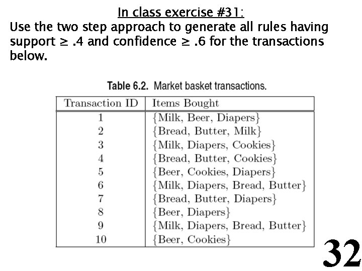
Two Step Approach: 1) Frequent Itemset Generation = Generate all itemsets whose support ≥ minsup 2) Rule Generation = Generate high confidence (confidence ≥ minconf ) rules from each frequent itemset, where each rule is a binary partitioning of a frequent itemset l Note: Frequent itemset generation is still computationally expensive and your book discusses algorithms that can be used 31

In class exercise #31: Use the two step approach to generate all rules having support ≥. 4 and confidence ≥. 6 for the transactions below. 32