Statistics 111 Lecture 9 Introduction to Inference Sampling

Statistics 111 - Lecture 9 Introduction to Inference Sampling Distributions for Counts and Proportions June 10, 2008 Stat 111 - Lecture 9 - Proportions 1

Administrative Notes • Homework 3 is due on Monday, June 15 th – Covers chapters 1 -5 in textbook • Exam on Monday, June 15 th • Review session on Thursday June 10, 2008 Stat 111 - Lecture 9 - Proportions 2

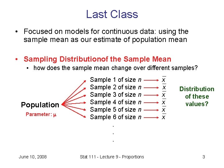
Last Class • Focused on models for continuous data: using the sample mean as our estimate of population mean • Sampling Distributionof the Sample Mean • how does the sample mean change over different samples? Population Parameter: June 10, 2008 Sample 1 of size n Sample 2 of size n Sample 3 of size n Sample 4 of size n Sample 5 of size n Sample 6 of size n. . . Stat 111 - Lecture 9 - Proportions x x x Distribution of these values? 3

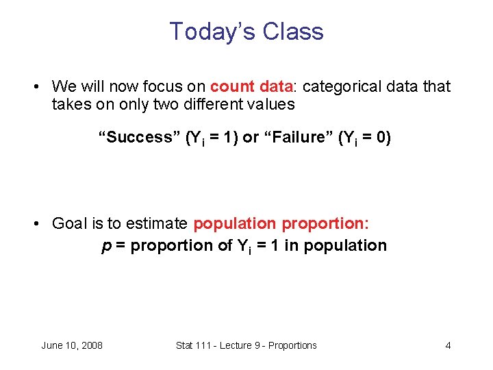
Today’s Class • We will now focus on count data: categorical data that takes on only two different values “Success” (Yi = 1) or “Failure” (Yi = 0) • Goal is to estimate population proportion: p = proportion of Yi = 1 in population June 10, 2008 Stat 111 - Lecture 9 - Proportions 4

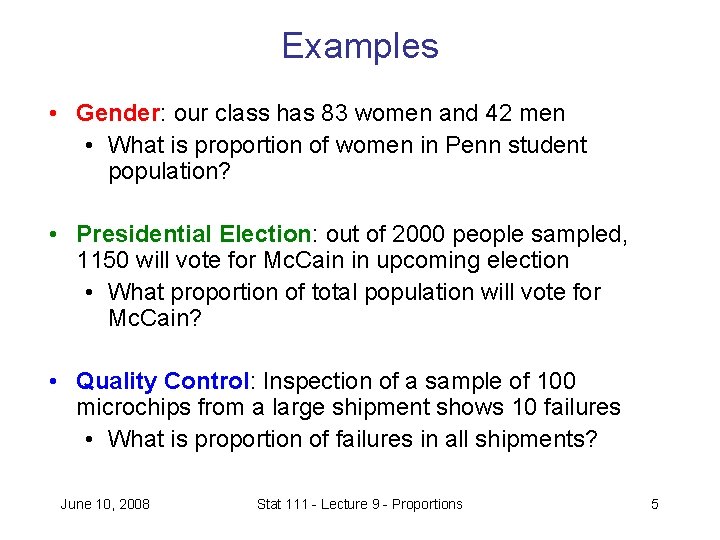
Examples • Gender: our class has 83 women and 42 men • What is proportion of women in Penn student population? • Presidential Election: out of 2000 people sampled, 1150 will vote for Mc. Cain in upcoming election • What proportion of total population will vote for Mc. Cain? • Quality Control: Inspection of a sample of 100 microchips from a large shipment shows 10 failures • What is proportion of failures in all shipments? June 10, 2008 Stat 111 - Lecture 9 - Proportions 5

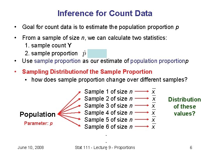
Inference for Count Data • Goal for count data is to estimate the population proportion p • From a sample of size n, we can calculate two statistics: 1. sample count Y 2. sample proportion = Y/n • Use sample proportion as our estimate of population proportionp • Sampling Distributionof the Sample Proportion • how does sample proportion change over different samples? Population Parameter: p June 10, 2008 Sample 1 of size n Sample 2 of size n Sample 3 of size n Sample 4 of size n Sample 5 of size n Sample 6 of size n. . Stat 111 - Lecture. 9 - Proportions x x x Distribution of these values? 6

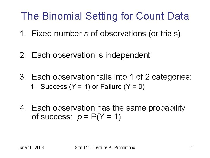
The Binomial Setting for Count Data 1. Fixed number n of observations (or trials) 2. Each observation is independent 3. Each observation falls into 1 of 2 categories: 1. Success (Y = 1) or Failure (Y = 0) 4. Each observation has the same probability of success: p = P(Y = 1) June 10, 2008 Stat 111 - Lecture 9 - Proportions 7

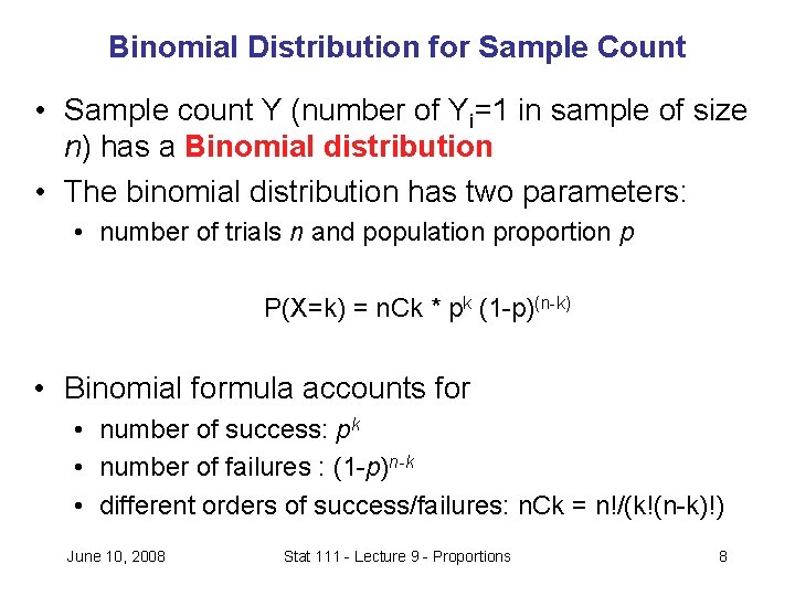
Binomial Distribution for Sample Count • Sample count Y (number of Yi=1 in sample of size n) has a Binomial distribution • The binomial distribution has two parameters: • number of trials n and population proportion p P(X=k) = n. Ck * pk (1 -p)(n-k) • Binomial formula accounts for • number of success: pk • number of failures : (1 -p)n-k • different orders of success/failures: n. Ck = n!/(k!(n-k)!) June 10, 2008 Stat 111 - Lecture 9 - Proportions 8

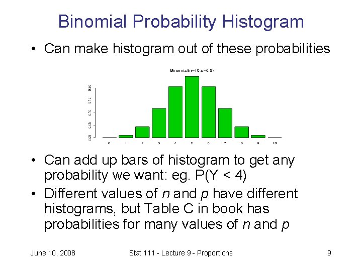
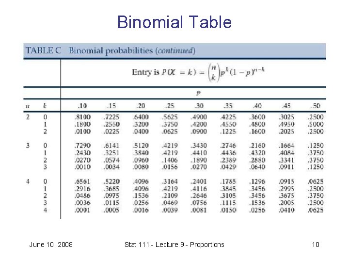
Binomial Probability Histogram • Can make histogram out of these probabilities • Can add up bars of histogram to get any probability we want: eg. P(Y < 4) • Different values of n and p have different histograms, but Table C in book has probabilities for many values of n and p June 10, 2008 Stat 111 - Lecture 9 - Proportions 9

Binomial Table June 10, 2008 Stat 111 - Lecture 9 - Proportions 10

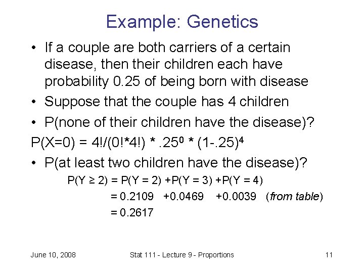
Example: Genetics • If a couple are both carriers of a certain disease, then their children each have probability 0. 25 of being born with disease • Suppose that the couple has 4 children • P(none of their children have the disease)? P(X=0) = 4!/(0!*4!) *. 250 * (1 -. 25)4 • P(at least two children have the disease)? P(Y ≥ 2) = P(Y = 2) +P(Y = 3) +P(Y = 4) = 0. 2109 +0. 0469 +0. 0039 (from table) = 0. 2617 June 10, 2008 Stat 111 - Lecture 9 - Proportions 11

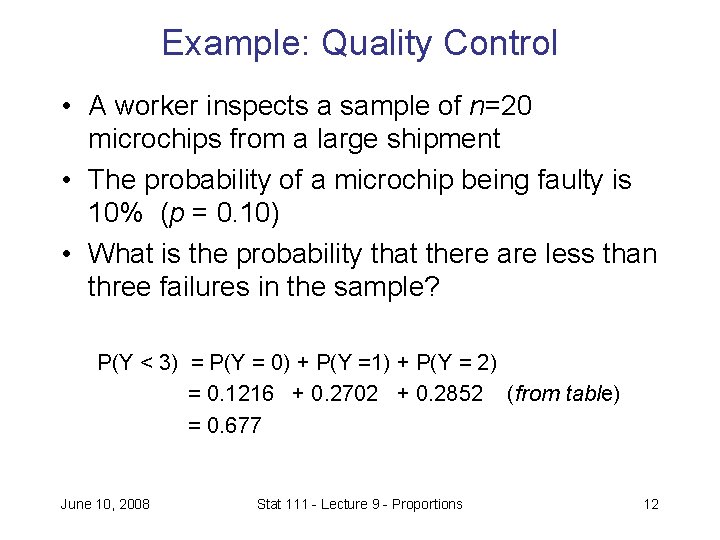
Example: Quality Control • A worker inspects a sample of n=20 microchips from a large shipment • The probability of a microchip being faulty is 10% (p = 0. 10) • What is the probability that there are less than three failures in the sample? P(Y < 3) = P(Y = 0) + P(Y =1) + P(Y = 2) = 0. 1216 + 0. 2702 + 0. 2852 (from table) = 0. 677 June 10, 2008 Stat 111 - Lecture 9 - Proportions 12

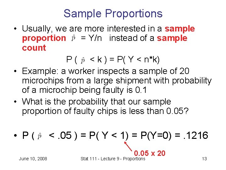
Sample Proportions • Usually, we are more interested in a sample proportion = Y/n instead of a sample count P ( < k ) = P( Y < n*k) • Example: a worker inspects a sample of 20 microchips from a large shipment with probability of a microchip being faulty is 0. 1 • What is the probability that our sample proportion of faulty chips is less than 0. 05? • P( June 10, 2008 <. 05 ) = P( Y < 1) = P(Y=0) =. 1216 0. 05 x 20 Stat 111 - Lecture 9 - Proportions 13

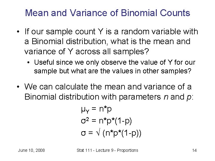
Mean and Variance of Binomial Counts • If our sample count Y is a random variable with a Binomial distribution, what is the mean and variance of Y across all samples? • Useful since we only observe the value of Y for our sample but what are the values in other samples? • We can calculate the mean and variance of a Binomial distribution with parameters n and p: μY = n*p σ2 = n*p*(1 -p) σ = √ (n*p*(1 -p)) June 10, 2008 Stat 111 - Lecture 9 - Proportions 14

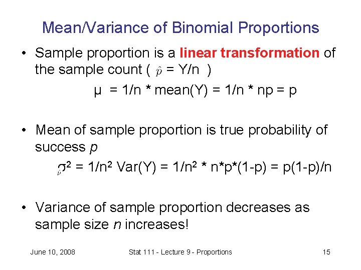
Mean/Variance of Binomial Proportions • Sample proportion is a linear transformation of the sample count ( = Y/n ) μ = 1/n * mean(Y) = 1/n * np = p • Mean of sample proportion is true probability of success p σ2 = 1/n 2 Var(Y) = 1/n 2 * n*p*(1 -p) = p(1 -p)/n • Variance of sample proportion decreases as sample size n increases! June 10, 2008 Stat 111 - Lecture 9 - Proportions 15

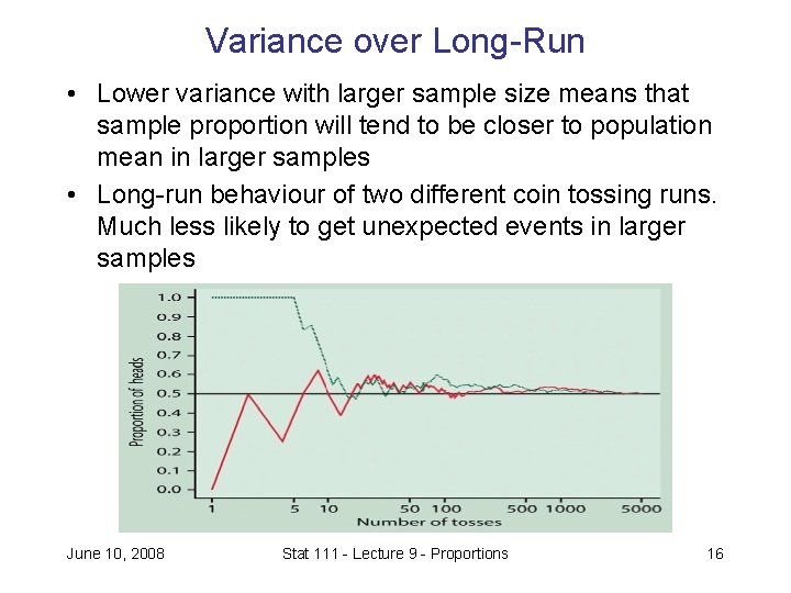
Variance over Long-Run • Lower variance with larger sample size means that sample proportion will tend to be closer to population mean in larger samples • Long-run behaviour of two different coin tossing runs. Much less likely to get unexpected events in larger samples June 10, 2008 Stat 111 - Lecture 9 - Proportions 16

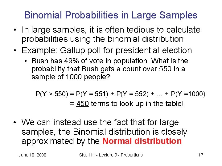
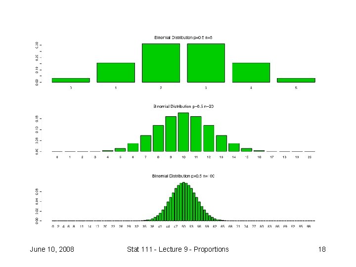
Binomial Probabilities in Large Samples • In large samples, it is often tedious to calculate probabilities using the binomial distribution • Example: Gallup poll for presidential election • Bush has 49% of vote in population. What is the probability that Bush gets a count over 550 in a sample of 1000 people? P(Y > 550) = P(Y = 551) + P(Y = 552) + … + P(Y =1000) = 450 terms to look up in the table! • We can instead use the fact that for large samples, the Binomial distribution is closely approximated by the Normal distribution June 10, 2008 Stat 111 - Lecture 9 - Proportions 17

June 10, 2008 Stat 111 - Lecture 9 - Proportions 18

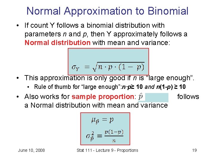
Normal Approximation to Binomial • If count Y follows a binomial distribution with parameters n and p, then Y approximately follows a Normal distribution with mean and variance: μY = n*p • This approximation is only good if n is “large enough”. • Rule of thumb for “large enough”: n·p≥ 10 and n(1 -p) ≥ 10 • Also works for sample proportion: = Y/n a Normal distribution with mean and variance June 10, 2008 Stat 111 - Lecture 9 - Proportions follows 19

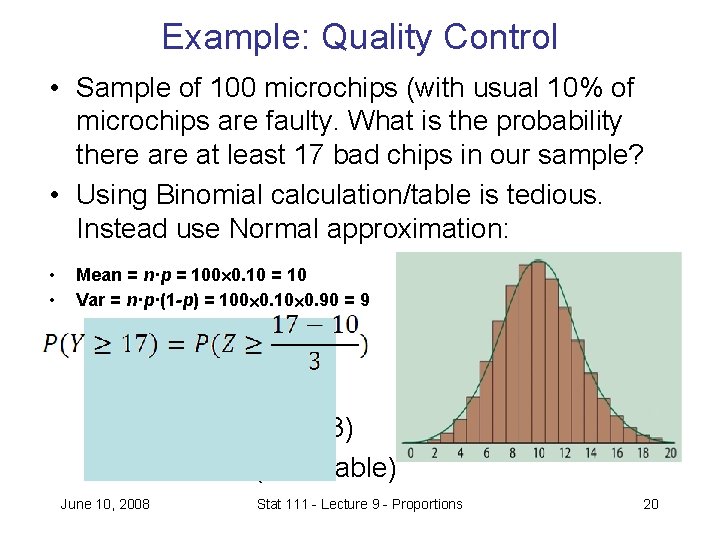
Example: Quality Control • Sample of 100 microchips (with usual 10% of microchips are faulty. What is the probability there at least 17 bad chips in our sample? • Using Binomial calculation/table is tedious. Instead use Normal approximation: • • Mean = n·p = 100 0. 10 = 10 Var = n·p·(1 -p) = 100 0. 10 0. 90 = 9 = P(Z ≥ 2. 33) =1 - P(Z ≤ 2. 33) = 0. 01 (from table) June 10, 2008 Stat 111 - Lecture 9 - Proportions 20

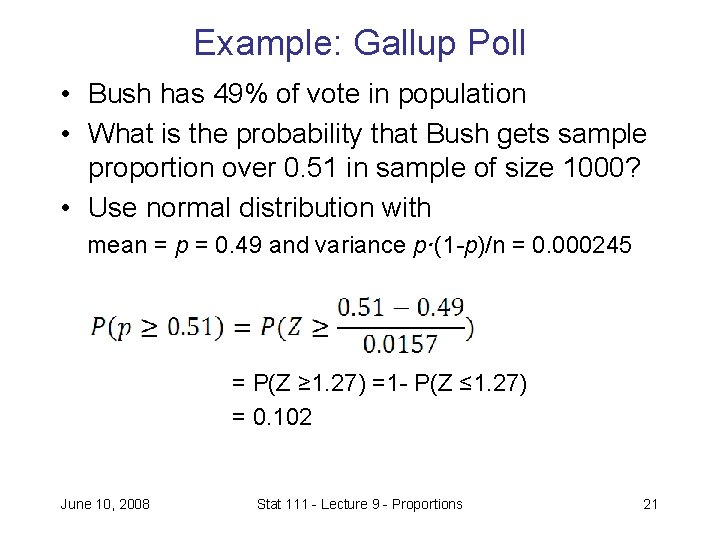
Example: Gallup Poll • Bush has 49% of vote in population • What is the probability that Bush gets sample proportion over 0. 51 in sample of size 1000? • Use normal distribution with mean = p = 0. 49 and variance p·(1 -p)/n = 0. 000245 = P(Z ≥ 1. 27) =1 - P(Z ≤ 1. 27) = 0. 102 June 10, 2008 Stat 111 - Lecture 9 - Proportions 21

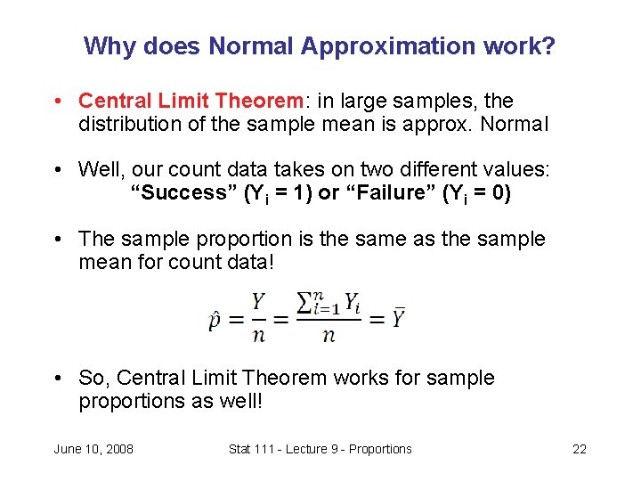
Why does Normal Approximation work? • Central Limit Theorem: in large samples, the distribution of the sample mean is approx. Normal • Well, our count data takes on two different values: “Success” (Yi = 1) or “Failure” (Yi = 0) • The sample proportion is the same as the sample mean for count data! • So, Central Limit Theorem works for sample proportions as well! June 10, 2008 Stat 111 - Lecture 9 - Proportions 22

Next Class - Lecture 10 • Review session on Wednesday/Thursday – Show up with questions! June 10, 2008 Stat 111 - Lecture 9 - Proportions 23