Statistics 1 The Normal Distribution The Standard Normal
Statistics 1 The Normal Distribution
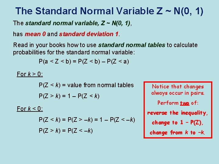
The Standard Normal Variable Z ~ N(0, 1) The standard normal variable, Z ~ N(0, 1), has mean 0 and standard deviation 1. Read in your books how to use standard normal tables to calculate probabilities for the standard normal variable: P(a < Z < b) = P(Z < b) – P(Z < a) For k > 0: P(Z < k) = value from normal tables P(Z > k) = 1 – P(Z < k) For k < 0: P(Z < k) = P(Z > –k) = 1 – P(Z < –k) P(Z > k) = P(Z < –k) Notice that changes always occur in pairs. Perform two of: reverse the inequality, change to 1 – P(Z), change from k to –k.
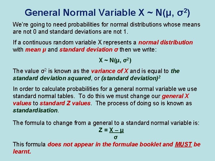
General Normal Variable X ~ N(μ, σ2) We’re going to need probabilities for normal distributions whose means are not 0 and standard deviations are not 1. If a continuous random variable X represents a normal distribution with mean μ and standard deviation σ then we write: X ~ N(μ, σ2) The value σ2 is known as the variance of X and is equal to the standard deviation squared, or (standard deviation)2 In order to calculate probabilities for a general normal variable we use standard normal tables. To do this we must change our general X values to standard Z values. The process of doing so is known as standardisation. The formula to change from a general to a standard normal variable is: Z=X–μ σ This formula does not appear in the formulae booklet and MUST be learnt.
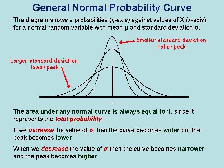
General Normal Probability Curve The diagram shows a probabilities (y-axis) against values of X (x-axis) for a normal random variable with mean μ and standard deviation σ. Smaller standard deviation, taller peak Larger standard deviation, lower peak μ The area under any normal curve is always equal to 1, since it represents the total probability If we increase the value of σ then the curve becomes wider but the peak becomes lower When we decrease the value of σ then the curve becomes narrower and the peak becomes higher
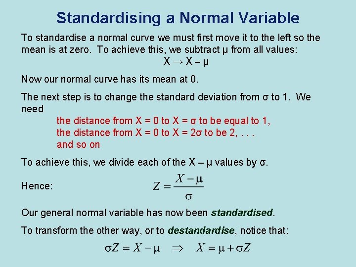
Standardising a Normal Variable To standardise a normal curve we must first move it to the left so the mean is at zero. To achieve this, we subtract μ from all values: X→X–μ Now our normal curve has its mean at 0. The next step is to change the standard deviation from σ to 1. We need the distance from X = 0 to X = σ to be equal to 1, the distance from X = 0 to X = 2σ to be 2, . . . and so on To achieve this, we divide each of the X – μ values by σ. Hence: Our general normal variable has now been standardised. To transform the other way, or to destandardise, notice that:
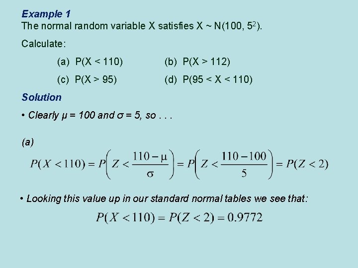
Example 1 The normal random variable X satisfies X ~ N(100, 52). Calculate: (a) P(X < 110) (b) P(X > 112) (c) P(X > 95) (d) P(95 < X < 110) Solution • Clearly μ = 100 and σ = 5, so. . . (a) • Looking this value up in our standard normal tables we see that:
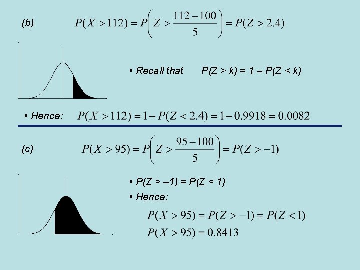
(b) • Recall that P(Z > k) = 1 – P(Z < k) • Hence: (c) • P(Z > – 1) = P(Z < 1) • Hence:
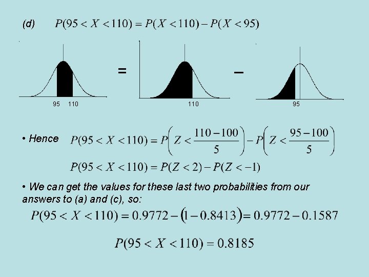
(d) = 95 110 – 110 95 • Hence • We can get the values for these last two probabilities from our answers to (a) and (c), so:
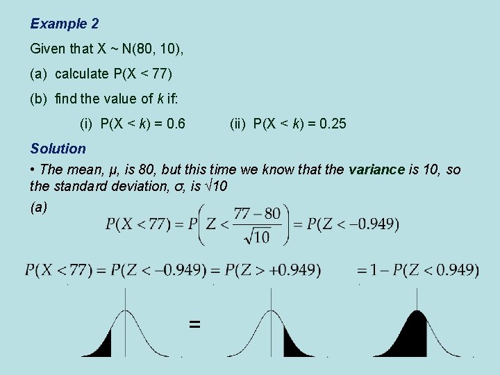
Example 2 Given that X ~ N(80, 10), (a) calculate P(X < 77) (b) find the value of k if: (i) P(X < k) = 0. 6 (ii) P(X < k) = 0. 25 Solution • The mean, μ, is 80, but this time we know that the variance is 10, so the standard deviation, σ, is √ 10 (a) =
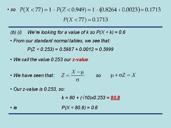
• so (b) (i) We’re looking for a value of k so P(X < k) = 0. 6 • From our standard normal tables, we see that: P(Z < 0. 253) = 0. 5987 + 0. 0012 = 0. 5999 • We call the value 0. 253 our z-value • We have seen that: so • Our z-value is 0. 253, so: k = 80 + (√ 10)x 0. 253 = 80. 8 • ie P(X < 80. 8) = 0. 6
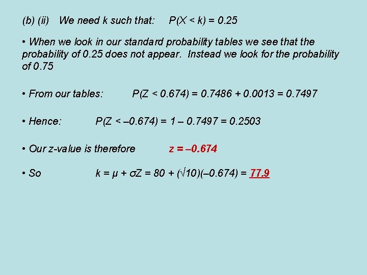
(b) (ii) We need k such that: P(X < k) = 0. 25 • When we look in our standard probability tables we see that the probability of 0. 25 does not appear. Instead we look for the probability of 0. 75 • From our tables: • Hence: P(Z < 0. 674) = 0. 7486 + 0. 0013 = 0. 7497 P(Z < – 0. 674) = 1 – 0. 7497 = 0. 2503 • Our z-value is therefore • So z = – 0. 674 k = μ + σZ = 80 + (√ 10)(– 0. 674) = 77. 9
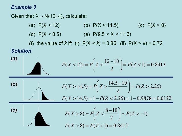
Example 3 Given that X ~ N(10, 4), calculate: (a) P(X < 12) (b) P(X > 14. 5) (d) P(X < 8. 5) (e) P(9. 5 < X < 11. 5) (c) P(X > 8) (f) the value of k if: (i) P(X < k) = 0. 85 (ii) P(X > k) = 0. 72 Solution (a) (b) (c)
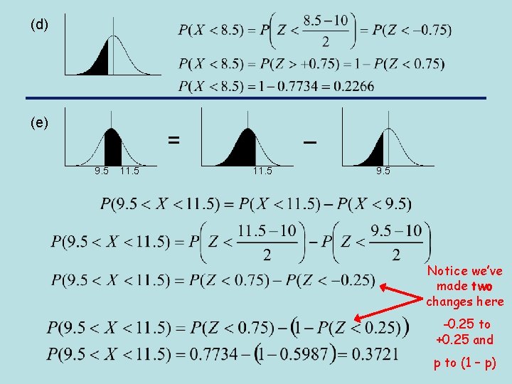
(d) (e) = 9. 5 11. 5 – 11. 5 9. 5 Notice we’ve made two changes here -0. 25 to +0. 25 and p to (1 – p)
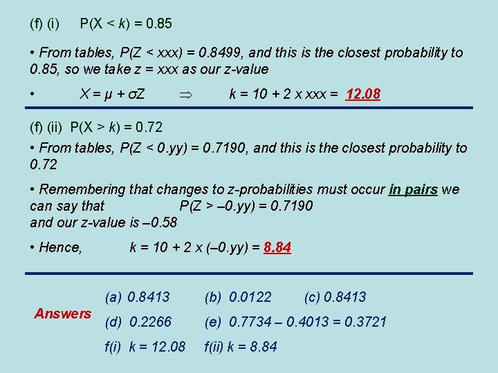
(f) (i) P(X < k) = 0. 85 • From tables, P(Z < xxx) = 0. 8499, and this is the closest probability to 0. 85, so we take z = xxx as our z-value • X = μ + σZ k = 10 + 2 x xxx = 12. 08 (f) (ii) P(X > k) = 0. 72 • From tables, P(Z < 0. yy) = 0. 7190, and this is the closest probability to 0. 72 • Remembering that changes to z-probabilities must occur in pairs we can say that P(Z > – 0. yy) = 0. 7190 and our z-value is – 0. 58 • Hence, Answers k = 10 + 2 x (– 0. yy) = 8. 84 (a) 0. 8413 (b) 0. 0122 (d) 0. 2266 (e) 0. 7734 – 0. 4013 = 0. 3721 f(i) k = 12. 08 f(ii) k = 8. 84 (c) 0. 8413
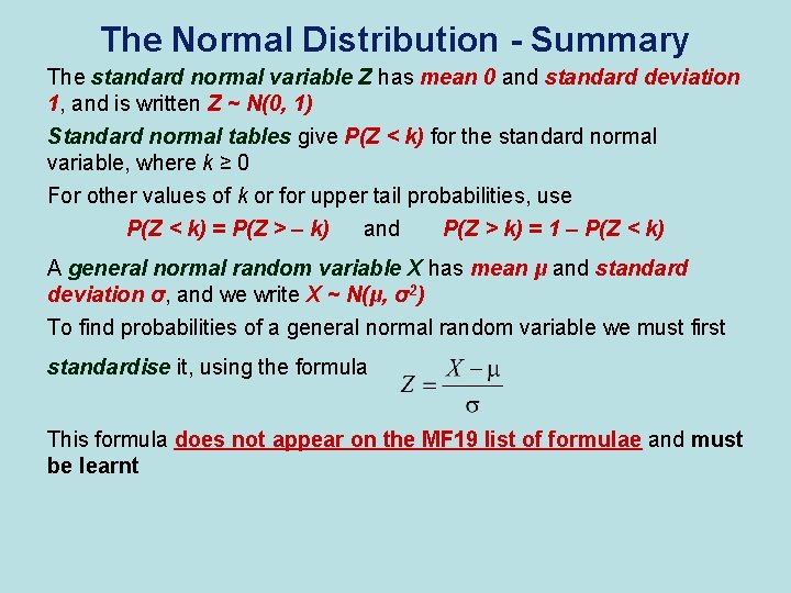
The Normal Distribution - Summary The standard normal variable Z has mean 0 and standard deviation 1, and is written Z ~ N(0, 1) Standard normal tables give P(Z < k) for the standard normal variable, where k ≥ 0 For other values of k or for upper tail probabilities, use P(Z < k) = P(Z > – k) and P(Z > k) = 1 – P(Z < k) A general normal random variable X has mean μ and standard deviation σ, and we write X ~ N(μ, σ2) To find probabilities of a general normal random variable we must first standardise it, using the formula This formula does not appear on the MF 19 list of formulae and must be learnt
- Slides: 15