Statistical Thermodynamics Lecture 13 Conformational Sampling MC and


 If Acceptance probability (probability of accepting move once")

 Connections between microscopic information such as atomic positions and velocities and")


 algorithms: velocity Verlet, position Verlet, leap frog, predictor-corrector, . . .")


 There are different methods")
 2) 3) 4) 5) Energy minimization Thermalization")
- Slides: 22
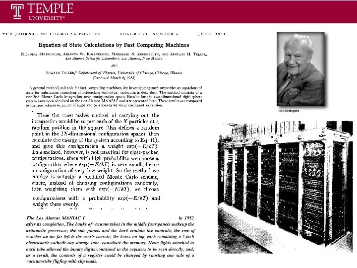
Statistical Thermodynamics Lecture 13: Conformational Sampling: MC and MD Dr. Ronald M. Levy ronlevy@temple. edu Contributions from Mike Andrec and Daniel Weinstock
Importance Sampling and Monte Carlo Methods Energy functions are useless without sampling methods • Knowing the energy of every point in a high-dimensional phase space is essential but not terribly informative • Thermodynamic quantities are averages over an ensemble over the entire phase space • We are often interested in the distribution of certain quantities (e. g. radius of gyration) averaged over all of the “uninteresting” degrees of freedom (aka “potentials of mean force”)
Thermodynamic quantities are averages over an ensemble over the entire phase space This could be evaluated by numerical integration over a grid, or by generating random points uniformly over phase space and estimating the integral by MC integration: In fact, the complete phase space may not be needed, since the velocity contributions can often be accounted for analytically. Then, we only need to consider the potential energy of conformational degrees of freedom.
These methods are generally hopeless for molecular systems: N is huge, Q is unknown, and most points in a uniform sampling have a very small value of the integrand. Frenkel & Smit (2002) Understanding Molecular Simulations, 2 nd Ed. , Academic Press
Importance Sampling by Markov Chain Monte Carlo Want to produce conformations distributed according to Given a current point i in configuration space, choose a subsequent point i+1 with transition probability ( i, i+1) that depends only on i. To get the correct sampling, it is sufficient that the transition probabilities satisfy microscopic reversibility: ( i) ( i, i+1) = ( i+1) ( i+1, i), or (flux i to j = flux j to i = equilibrium) j i
Proposal probability (probability of picking move) If Acceptance probability (probability of accepting move once it has been selected) (symmetric MC scheme) one valid choice: j i 4
The “classic” Metropolis algorithm • Pick a degree of freedom x • Displace x by a uniformly distributed random number in range ± • Calculate the potential energy difference between the current state i and the proposed displaced state j • Accept the move if • Otherwise draw random number and accept if “Reject” does not mean “omit”… j i
Molecular Dynamics (MD) Connections between microscopic information such as atomic positions and velocities and macroscopic observables is through statistical mechanics. In statistical mechanics, averages are defined as ensemble averages However, in MD simulations, we calculate time averages Ergodic Hypothesis
Historical Background 1956: Alder and Wainwright MD method developed to study interactions of hard spheres 1964: Rahman first simulation with realistic potential - liquid Argon 1971: Stillinger and Rahman first simulation of realistic system - liquid water 1977: Mc. Cammon, Gelin, and Karplus first protein simulation - BPTI
System of N particles Positions of the N particles, Velocities of the N particles Energy(E) of the system Kinetic Energy Potential Energy, V( r) System Temperature Microcanonical ensemble (constant NVE) closed system - no energy enters or leaves energy conservation used to check MD algorithm
Newton’s Equations of Motion The forces are complicated functions of the coordinates, non-linear functions of position, so the set of 3 N coupled differential equations cannot be solved analytically.
Numerical Integration of the Equations of Motion The integrator is the heart of an MD algorithm Given molecular position, velocities and other dynamic information at time t, we attempt to obtain the positions, velocities, etc. at a later time t+δt to a sufficient degree of accuracy Finite difference method: Not very accurate, leads to divergences unless δt is made very small.
Better O(δt 2) algorithms: velocity Verlet, position Verlet, leap frog, predictor-corrector, . . . ? Allen and Tildesley. Computer Simulations of Liquids. 1987.
The Liouville operator For any property A: q-component propagates coordinates in time: p-component propagates momenta in time:
Trotter expansion In general Because Lq and Lp don't commute However if δt is sufficiently small: Trotter
r. RESPA Defines integrator made of P steps each made of 3 operations: 1. Propagate momenta to δt/2: 1. Propagate momenta to δt:
r. RESPA equivalent to velocity Verlet Most other integrators can be derived using different forms of short time expansions of the Liouville propagator
Choice of Time Step should be small enough for trajectories to be close to exact Energy Conservation is used as a criteria for choosing the time step signals good energy conservation We want to use a time step that minimizes computational time, while maintaining Energy Conservation The faster time scales control the time step δt to use. To integrate vibrations need to choose δt much smaller than 1 fs
Multiple time step r. RESPA Decompose total force in a fast component (covalent interactions inexpensive) and a slow component (non-bonded interactions expensive): Short time propagator: Then break up inner fast propagator using a shorter time step: Fast forces are applied N times in the inner loop allowing larger time step in outer loop.
Constant Temperature Molecular Dynamics Canonical ensemble (constant N, V, T) There are different methods for constant temperature MD • Andersen velocity resampling • Nosé-Hoover thermostat (extended system) • the system is coupled to extra degrees of freedom which simulate heat bath. Original system is canonical, extended system is microcanonical • Langevin thermostat. Periodically atomic velocities are stochastically perturbed based on friction coefficient and relaxation time. • Berendsen thermostat (velocity rescaling – non canonical)
Typical Organization of a MD simulation 1) 2) 3) 4) 5) Energy minimization Thermalization Equilibration Production Trajectory Analysis