Statistical Thermodynamics Binding equilibria I DDM FEP BEDAM

Statistical Thermodynamics Binding equilibria I: DDM, FEP, BEDAM

Protein-ligand binding free energy ΔG = ? HIV Integrate • Quantitatively evaluation of the binding free energy between protein and ligand is a key task in the computational biology. • Predicting the binding free energy have great practical values in pharmaceutical drug design.

Equilibrium binding constant and binding free energy • In chemical equilibrium condition: [L], [R], [LR] are the concentration of the free ligand, free receptor and bound ligand-receptor complex. Kb is the binding constant for the reaction:

Thermodynamic cycle to calculate binding free energy ΔF 0 decoupling ligand in pure water ΔFwater we call it double decoupling method ΔFprotein ΔFgas = 0 recoupling ligand in protein problem will arise in this step since it is not reversible

Thermodynamic cycle to calculate binding free energy with restraint Protein (P) Ligand (L) Complex (PL) ΔF 0 Lelec+vdw ΔFwater PLelec+vdw ΔFprotein, restraint L PLrestraint+elec+vdw ΔFgas, restraint ΔFprotein ΔFgas= 0 Lrestraint PLrestraint

Calculation of binding free energy with restraint

Calculation of free energy to restrain ligand in gas phase • The relative distance of ligand is a function of ra. A(a. A), θA(ba. A) and ϕA(cba. A) • The relative orientation of ligand is a function of θB(a. AB), ϕB(ba. AB) and ϕC(a. ABC) separate the degree of freedom of the ligand into internal part and external part rigid rotator approximation

Free energy perturbation method • The main idea: One starts with an initial system, called the unperturbed or reference system. The system of interest, called the target system, is represented in terms of a perturbation to the reference system.

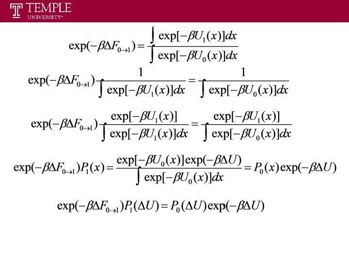
Probability density function P 0 of finding the reference system in a state defined by x: Fundamental formula for the transformation 0 1: • In this formula, ΔU(x) = U 1(x) – U 0(x) is the difference in potential between target and reference system, and the average is over the ensemble of the initial state corresponding to reference system with potential U 0(x) • Similarly, the free energy difference can also be written in terms of an average over the ensemble of the final state corresponding to target system with potential U 1(x)

The density of states and potential distribution theorem if If we define: One dimensional integral over the energy difference

• If U 0 and U 1 were the functions of a sufficient number of identically distributed random variables, then ΔU would be Gaussian distributed, which is a consequence of the central limit theorem. • In practice, P 0(ΔU) deviates somewhat from the ideal Gaussian, but still has a “Gaussian-like” shape. • The integrand, exp(-βΔU)* P 0(ΔU), is shifted to the left. • This indicates the value of the integral depends on the low-energy tail of distribution

Here we define: • We note that exp(-βΔU)P 0(ΔU) is a Gaussian, as is P 0(ΔU), but is not normalized and shifted toward low ΔU by βσ2. • This means accurate estimation of ΔA is possible only if the probability distribution in the low-ΔU region is sufficiently well know up to 2 standard deviations from the peak of exp(-βΔU)P 0(ΔU) or βσ2+2 standard deviations from the peak of P 0(ΔU). • If σ is small, equal to k. BT, 95% of the sampled values of ΔU are within 2σ of the peak of exp(-βΔU)P 0(ΔU) at room temperature. If σ is large, for example equal to 4 k. BT, this percentage drops to 5%. Evaluate the integration analytically: Notice: use of this analytical expression can be successful only if P 0(ΔU) is a narrow function of ΔU and P 0(ΔU) is a Gaussian distribution.

A Pictorial Representation of Free Energy Calculation • Accurate estimates of free energy differences can only achieved in condition that the target system is sufficient similar to the reference system. • Important regions in phase space: volumes that encompass configurations of the system with highly probable energy values. • If the important regions of reference system and target system do not overlap --- very bad sampling. • If the important region of target system is a subset of important region of reference system --- good sampling. • If the important region of reference overlaps only a part of that of target --- poor sampling • If the two important regions do not overlap or overlap only partially, it is necessary to use the stratification to enhance sampling

Free Energy Calculation --- Staging • The difficulty in applying FEP formula can be circumvented through staging strategy. • Construction of several intermediate states between reference and target state such that P(ΔUi, i+1) for two consecutive states i and i+1 sampled at state i is sufficiently narrow for the direct evaluation of the corresponding free energy difference ΔAi, i+1. • With N-2 intermediate states, • Intermediate states do not need to be physically meaningful, they do not have to correspond to systems that actually exist.

Free Energy Calculation --- formula • The potential energy can be considered to be a function of some parameter λ. • λ can be defined between 0 and 1, such that λ = 0 for reference state and λ = 1 for target state. • Dependence of hybrid potential energy on λ : ΔU is the perturbation potential energy, equal to U 1 -U 0. • If N-2 intermediate states are created to link the reference and target states, such that λ 1 = 0 and λN = 1: with Δλi =λi+1 -λi Total free energy difference:

Important concept in Free Energy Calculation : Order parameter • Order parameter: They are collective variables used to describe transformations from the reference system to the target one. order parameter: distance order parameter: dihedral • An order parameter may or may not correspond to the path along which the transformation takes place in nature, and would be called the reaction coordinate if such were the case. • There is more than one way to define an order parameter. The choice of order parameters may have a significant effect on the efficiency and accuracy of free energy calculations.

Example: Relative binding free energies for ligands • In the case of seeking potential inhibitors of a target protein, determining relative binding free energies for a series of ligands is required. This can be handled by repeating the absolute binding free energy calculation for each ligand of interest. ΔFXLC = -6. 93 kcal/mol Ligand XLC Protein FXa ΔFXLD = -9. 98 kcal/mol Ligand XLD Protein FXa ΔΔFcal = ΔFXLD – ΔFXLC = -3. 05 kcal/mol. Match well with ΔΔFexp = -2. 94 kcal/mol

Alchemical transformations - FEP protein + ligand A ΔFAbinding protein ΔF 0 mutation protein + ligand B ligand ΔF 1 mutation ΔFBbinding protein ligand • There is an alternate pathway for calculations of relative binding free energies. Mutation of ligand A into ligand B in both the bound and the free states, following a different thermodynamic cycle. • Example: In the mutation of ethane into methanol, the former serves as the common topology. As the carbon atom is transformed into oxygen, two hydrogen atoms of the methyl moiety are turned into non-interacting, “ghost” particles by annihilating their point charges and van der Waals parameters.