Statistical tests to observe the statistical significance of

Statistical tests to observe the statistical significance of qualitative variables (Chisquare, Fisher’s exact & Mac Nemar’s chisquare tests) Dr. Shaikh Shaffi Ahamed Ph. D. , Associate Professor Dept. of Family & Community Medicine

Types of Categorical Data Qualitative/Categorical Data Nominal Categories Ordinal Categories

Types of Analysis for Categorical Data Type of Analysis Analytic Descriptive Rate and Ratio Confidence Interval and Test of Significance

Contingency Tables Nominal Variables 2 X 2 Tables Pearson’s Chi-Square Yates Corrected Chi-Square R X C Tables Pearson’s Chi-Square Fisher’s Exact Test Co-efficient of Contingency Several 2 X 2 Tables Phi & Cramer’s V Goodman and Kruskal’s Lambda Ordinal Variables Matched Variables R X C Tables R X R Kendall’s Tau b & c Somer’s d Goodman and Kruskal’s Gamma Mc. Nemar Chi-Square

Choosing the appropriate Statistical test n Based on the three aspects of the data Types of variables n Number of groups being compared & n Sample size n
 Chi-square test: Study variable: Qualitative Outcome variable: Qualitative Comparison: two")
Statistical test (cont. ) Chi-square test: Study variable: Qualitative Outcome variable: Qualitative Comparison: two or more proportions Sample size: > 20 Expected frequency: > 5 Fisher’s exact test: Study variable: Qualitative Outcome variable: Qualitative Comparison: two proportions Sample size: < 20 Macnemar’s test: (for paired samples) Study variable: Qualitative Outcome variable: Qualitative Comparison: two proportions Sample size: Any

Chi-square test Purpose To find out whether the association between two categorical variables are statistically significant Null Hypothesis There is no association between two variables
 Figure for")
Chi- Square [ S 2 = X = ( o - e) Figure for Each Cell e ] 2

1. The summation is over all cells of the contingency table consisting of r rows and c columns 2. O is the observed frequency ^ 3. E is the expected frequency ^ E= total of column in total of row in • which the cell lies (total of all cells) reject Ho if 2 > 2. , df where df = (r-1)(c-1) (O - E )2 2 = ∑ E 4. The degrees of freedom are df = (r-1)(c-1)

Requirements n Prior to using the chi square test, there are certain requirements that must be met. n n The data must be in the form of frequencies counted in each of a set of categories. Percentages cannot be used. The total number observed must be exceed 20.

Requirements n n The expected frequency under the H 0 hypothesis in any one fraction must normally be less than 5. All the observations must be independent of each other. In other words, one observation must not have an influence upon another observation.
 TESTING FOR HOMOGENEITY")
APPLICATION OF CHI-SQUARE TEST n n n TESTING INDEPENDCNE (or ASSOCATION) TESTING FOR HOMOGENEITY TESTING OF GOODNESS-OF-FIT

Chi-square test n n Objective : Smoking is a risk factor for MI Null Hypothesis: Smoking does not cause MI D (MI) No D( No MI) Total Smokers 29 21 50 Non-smokers 16 34 50 Total 45 55 100

Chi-Square test MI Non-MI 29 Smoker O 21 O E 16 Non-Smoker O E 34 O E E

Chi-square test MI 29 Non-MI 21 Smoker O 50 O E E 16 34 Non-smoker O 50 O E 45 E 55 100

Chi-square test MI Non-MI 29 21 Smoker O E 22. 5 O 16 E 34 Non-smoker O 50 50 X 45 22. 5 = 100 50 O E 45 E 55 100

Chi-square test MI No MI 29 smoker O E 22. 5 O E 27. 5 34 16 Non smoker 50 21 22. 5 O O E 45 50 27. 5 E 55 100
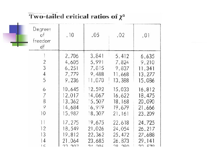
 (c-1) = (2 -1) =1 Critical Value")
Chi-Square Degrees of Freedom df = (r-1) (c-1) = (2 -1) =1 Critical Value (Table A. 6) = 3. 84 X 2 = 6. 84 Calculated value(6. 84) is greater than critical (table) value (3. 84) at 0. 05 level with 1 d. f. f Hence we reject our Ho and conclude that there is highly statistically significant association between smoking and MI.

Association between Diabetes and Heart Disease? n Background: Contradictory opinions: n 1. A diabetic’s risk of dying after a first heart attack is the same as that of someone without diabetes. There is no association between diabetes and heart disease. vs. n 2. Diabetes takes a heavy toll on the body and diabetes patients often suffer heart attacks and strokes or die from cardiovascular complications at a much younger age. n n So we use hypothesis test based on the latest data to see what’s the right conclusion. There a total of 5167 patients, among which 1131 patients are nondiabetics and 4036 are diabetics. Among the non-diabetic patients, 42% of them had their blood pressure properly controlled (therefore it’s 475 of 1131). While among the diabetic patients only 20% of them had the blood pressure controlled (therefore it’s 807 of 4036).

Association between Diabetes and Heart Disease? n Data Controlled Uncontrolled Total Non-diabetes 475 656 1131 Diabetes 807 3229 4036 Total 1282 3885 5167

Association between Diabetes and Heart Disease? Data: Diabetes: 1=Not have diabetes, 2=Have Diabetes Control: 1=Controlled, 2=Uncontrolled

Association between Diabetes and Heart Disease?

Association between Diabetes and Heart Disease? Hypothesis test: H 0: There is no association between diabetes and heart disease. (or) Diabetes and heart disease are independent. vs HA: There is an association between diabetes and heart disease. (or) Diabetes and heart disease are dependent. --- Assume a significance level of 0. 05

Association between Diabetes and Heart Disease? SPSS Output

Association between Diabetes and Heart Disease? ---The computer gives us a Chi-Square Statistic of 229. 268 ---The computer gives us a p-value of. 000 (<0. 0001) --- Because our p-value is less than alpha, we would reject the null hypothesis. --- There is sufficient evidence to conclude that there is an association between diabetes and heart disease.

Chi- square test Find out whether the gender is equally distributed among each age group Gender Male Female Total <30 60 (60) 40 (40) 100 Age 30 -45 20 (30) 30 (20) 50 >45 40 (30) 10 (20) 50 Total 120 80 200
 To test similarity between frequency distribution or group. It is")
Test for Homogeneity (Similarity) To test similarity between frequency distribution or group. It is used in assessing the similarity between nonresponders and responders in any survey Age (yrs) <20 Responders Non-responders Total 76 (82) 20 (14) 96 20 – 29 288 (289) 50 (49) 338 30 -39 312 (310) 51 (53) 363 40 -49 187 (185) 30 (32) 217 >50 77 (73) 9 (13) 86 Total 940 160 1100

Example n The following data relate to suicidal feelings in samples of psychotic and neurotic patients: Psychotics Neurotics Suicidal feelings Total 2 6 8 No suicidal feelings 18 14 32 Total 20 20 40

Example n The following data compare malocclusion of teeth with method of feeding infants. Normal teeth Malocclusion Breast fed 4 16 Bottle fed 1 21

Fisher’s Exact Test: n The method of Yates's correction was useful when manual calculations were done. Now different types of statistical packages are available. Therefore, it is better to use Fisher's exact test rather than Yates's correction as it gives exact result.

What to do when we have a paired samples and both the exposure and outcome variables are qualitative variables (Binary).

Problem n n A researcher has done a matched casecontrol study of endometrial cancer (cases) and exposure to conjugated estrogens (exposed). In the study cases were individually matched 1: 1 to a non-cancer hospitalbased control, based on age, race, date of admission, and hospital.

Mc. Nemar’s test Situation: Two paired binary variables that form a particular type of 2 x 2 table e. g. matched case-control study or cross-over trial

Data

can’t use a chi-squared test - observations are not independent - they’re paired. we must present the 2 x 2 table differently each cell should contain a count of the number of pairs with certain criteria, with the columns and rows respectively referring to each of the subjects in the matched pair the information in the standard 2 x 2 table used for unmatched studies is insufficient because it doesn’t say who is in which pair - ignoring the matching

Data

We construct a matched 2 x 2 table:

Formula The odds ratio is: f/g The test is: Compare this to the 2 distribution on 1 df

P <0. 001, Odds Ratio = 43/7 = 6. 1 p 1 - p 2 = (55/183) – (19/183) = 0. 197 (20%) s. e. (p 1 - p 2) = 0. 036 95% CI: 0. 12 to 0. 27 (or 12% to 27%)
 (c-1) = (2 -1) =1 Critical")
n n Degrees of Freedom df = (r-1) (c-1) = (2 -1) =1 Critical Value (Table A. 6) = 3. 84 n n n X 2 = 25. 92 Calculated value(25. 92) is greater than critical (table) value (3. 84) at 0. 05 level with 1 d. f. f Hence we reject our Ho and conclude that there is highly statistically significant association between Endometrial cancer and Estrogens.

Stata Output | Controls | Cases | Exposed Unexposed | Total -----------------+-----------Exposed | 12 43 | 55 Unexposed | 7 121 | 128 -----------------+-----------Total | 19 164 | 183 Mc. Nemar's chi 2(1) = 25. 92 Prob > chi 2 = 0. 0000 Exact Mc. Nemar significance probability = 0. 0000 Proportion with factor Cases. 3005464 Controls. 1038251 ----difference. 1967213 ratio 2. 894737 rel. diff. . 2195122 odds ratio 6. 142857 [95% Conf. Interval] ----------. 1210924. 2723502 1. 885462 4. 444269. 1448549. 2941695 2. 739772 16. 18458 (exact)
:")
In Conclusion ! When both the study variables and outcome variables are categorical (Qualitative): Apply (i) Chi square test (ii) Fisher’s exact test (Small samples) (iii) Mac nemar’s test ( for paired samples)
- Slides: 43