Statistical Techniques Robyn Valerie CSC 426 51415 Outline

Statistical Techniques Robyn & Valerie CSC 426 5/14/15

Outline 1. 2. 3. 4. 5. Motivation Background & Getting to Know Your Data Pre-processing Inferential Statistics (Analysis) Inference / Results

Motivation Why are we here?

Motivation • • • Effectively conduct research Know what statistics to use before collecting data To better read journal articles To further develop critical and analytic thinking To be an informed consumer
 conclusion validity • Degree to which conclusions we reach about relationships in data")
(Statistical) conclusion validity • Degree to which conclusions we reach about relationships in data are reasonable • Is there actually a relationship ? ? ? ▫ Conclude there is a relationship when there isn’t one ▫ Conclude there isn’t a relationship when there is one!

Threats • reliability of measures/observations • statistical power ▫ Sample size ▫ Alpha level (Type I) ▫ Power (Type II) • fishing and the error rate problem • violated assumptions of statistical tests

Get to know your data With some background

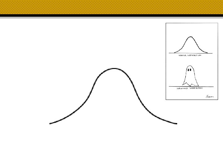
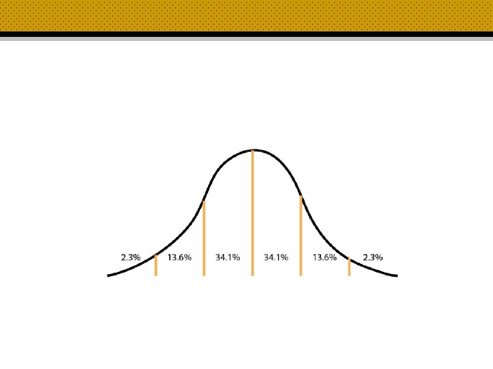
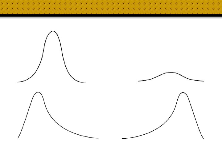
Get to Know Your Data • Population vs. Sample • Independent vs. Dependent Variables • Data Types • Descriptives • Distributions • Correlation

Population vs Sample

Data types • Nominal • Ordinal • Interval/Ratio
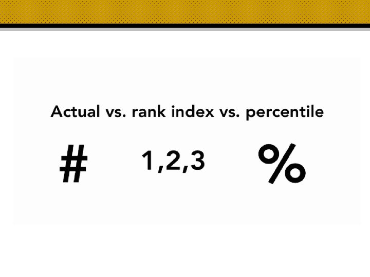

GDP USA • $16, 768, 100, 000 • Rank: 1 • Percentile: 100 th CYPRUS • $22, 767, 000 • Ranks: 102 • Percentile: 46 th
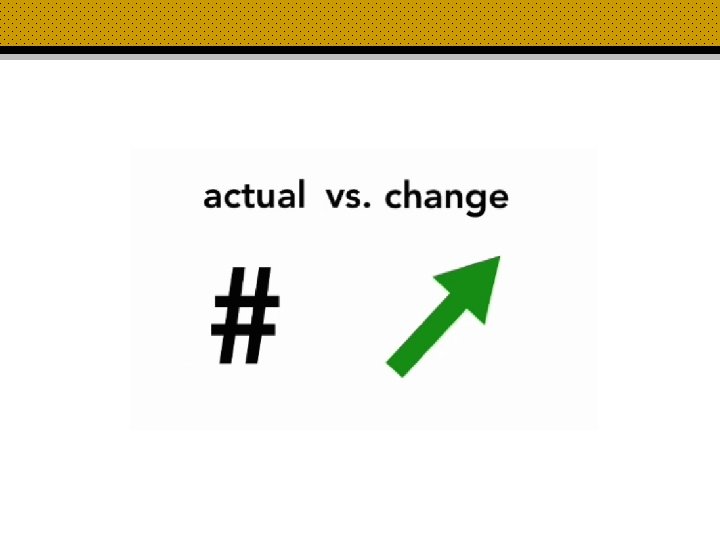

Actual vs. change Country GDP Growth Japan $4. 7913 Trillion 2. 26% China $1. 1838 Trillion 8. 43%

Descriptive Statistics Univariate Bivariate Describes the distribution of a single variable Describes the relationship between pairs of variables • • • Central Tendency Five Number Summary Dispersion Measures of Spread Shape • Cross-tabulations and Contingency Tables • Graphical Representation via Scatterplots • Quantitative Measures of Dependence

Measures of Central Tendency Hockey Player Points Scored 6, 7, 13, 17, 20, 22, 24, 24, 25, 27, 28, 35, 36, 50 Mean ~ 24 Median 24 Mode 24

Measures of Central Tendency Hockey Player Points Scored 6, 7, 13, 17, 20, 22, 24, 24, 25, 27, 28, 35, 36, 50, 517 Mean ~ 54 Median 24 Mode 24

Five Number Summary / Measures of Dispersion / Measures of Spread Hockey Player Points Scored 6, 7, 13, 17, 20, 22, 24, 24, 25, 27, 28, 35, 36, 50 Minimum First Quartile Median • Range = Max - Min = 44 • Standard Deviation (SD) = 11. 2 • Variance = s^2 = 126. 4 Third Quartile Maximum

Correlation

Correlation vs. Causation Correlation does not imply causation Correlation does not imply causation

Data preparation / pre-processing Cleaning, integrating and transforming your data!

Dirty Data • Incomplete ▫ occupation=“ ” • Noisy Major threats to conclusion validity ▫ Salary=“-10” • Inconsistent: ▫ Age=“ 42” Birthday=“ 03/07/1997” ▫ Was rating “ 1, 2, 3”, now rating “A, B, C” ▫ Discrepancy between duplicate records

Forms of data pre-processing • Cleaning • Integration • Transformation • Reduction
 �Ignore �Constant: “unknown”, a")
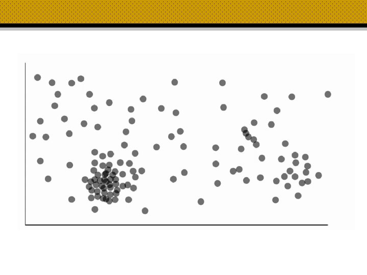
Data cleaning ▫ Fill in missing values (manual vs. automatic) �Ignore �Constant: “unknown”, a new class? ! �Attribute mean (of entire set or subset) �Most probable value: inference-based ▫ Identify outliers and smooth out noisy data �Binning method �Clustering �Combined computer and human inspection �Regression ▫ Correct inconsistent data ▫ Resolve redundancy caused by data integration

Outlier Detection Cluster Analysis

Regression y Y 1 y=x+1 Y 1’ X 1 x

Data Integration • Remove redundancies ▫ Correlational analysis • Integrate Schemas • Detec, resolve value conflicts

Data Transformation •
 • normalization by decimal scaling Where")
Normalization • min-max normalization • z-score normalization (standardization) • normalization by decimal scaling Where j is the smallest integer such that Max(| |)<1
 Parametric and Non-parametric")
Inferential Statistics (Analysis) Parametric and Non-parametric

Parametric vs Nonparametric • Interval or ratio scales • Data fall into a normal distribution • More complex and powerful analysis • Check for analysis methods what assumptions are absolutely necessary for use • Do not violate assumptions Ordinal Bi-modal or skewed distributions Less assumptions in general Number of parameters grows with the training data • More robust • Simpler, can be used when less is known about the application • • • Downside - A larger sample size may be need to draw conclusions with the same confidence
 •")
Inferential procedures Purpose Parametric Non-parametric Sig. difference between 2 MCTs Student’s t-test (means) • • Sig. difference between 3 or more MCTs ANOVA Kruskal-Wallis test Sig. diff among MCT while controlling for covariate ANCOVA Is r larger than it would be by chance? T-test for r Mann-Whitney U (median) Wilcoxon signed rank test (median, correlated) Fisher’s exact test How closely observations match expected (freq. or probability) MCT: Measure of central tendency (mean, median, mode)
 Experimental Design Analysis")
So you designed an experiment, what now? Quasiexperimental (no random assignment) Experimental Design Analysis Two-group posttest-only randomized T-test One-way ANOVA Factorial ANOVA Randomized block design ANOVA with blocking Analysis of Covariance ANCOVA Nonequivalent Groups (NEGD) Reliability-corrected ANCOVA Regression-Discontinuity Polynomial regression Regression Point Displacement ANCOVA variant
 •")
General Linear Model (GLM) •

Checking assumptions: iid residuals

Checking assumptions: Normality via Q-Q plots

Hypothesis/significance testing • Testing whether claims or hypotheses regarding a population are likely to be true • State hypotheses (H 0 and Ha) ▫ H 0 assumed to be true but we think it is wrong ▫ Ha contradicts H 0 (what we think is wrong about H 0) • Set criteria for decision ▫ amount of error we wish to accept • Compute test statistic ▫ mathematical formula that allows researchers to determine the likelihood of obtaining sample outcomes if the null hypothesis were true • Make a decision ▫ reject or fail to reject null hypothesis

t vs. z

One sample analysis Confidence limits for the mean One-sample t-test • •

Two sample t-tests • • Not paired ▫ Pooled variance �Assume populations have the same variance ▫ Not pooled variance

Example: Run time Alg 1 Alg 2 d 1. 2 1. 4 0. 2 -1. 27 4. 2 2. 3 1. 9 0. 43 2. 3 1. 2 -0. 27 3. 4 2. 1 1. 3 0. 17 4. 1 1. 3 2. 8 1. 33 4. 2 3. 2 1 -0. 47 2. 1 1. 2 0. 9 -1. 43 3. 2 1. 3 1. 9 0. 43 4. 2 2. 1 0. 63 • Statistic Value n 9 1. 47 s 0. 28

Non-parametric Less assumptions in general No assumption made to the distribution of the data Number of parameters grows with the training data Used for data that takes on a ranked order without clear numerical interpretation • More robust • Simpler, can be used when less is known about the application • • • Downside - A larger sample size may be need to draw conclusions with the same confidence

Parametric vs Nonparametric • Interval or ratio scales • Data fall into a normal distribution • More complex and powerful analysis • Check for analysis methods what assumptions are absolutely necessary for use • Do not violate assumptions Ordinal Bi-modal or skewed distributions Less assumptions in general Number of parameters grows with the training data • More robust • Simpler, can be used when less is known about the application • • • Downside - A larger sample size may be need to draw conclusions with the same confidence

Ordinal / Not Interval Experimental Design Two-group posttest-only randomized experiment Equivalent to independent samples T-test Analysis Mann-Whitney U Two-group posttest-only Wilcoxon Signed-Rank randomized experiment Test Equivalent to dependent samples T-test Three or more groups Equivalent to ANOVA Kruskal-Wallis Test

Two Dichotomous Variables Experimental Design Analysis Nominal Variables Odds Ratio Significant Correlation Equivalent to T-test for Pearson’s r Nominal or Ordinal Fisher’s Exact Test Significant Correlation Small sample size Equivalent to T-test for Pearson’s r

• Determines how closely observed frequencies or probabilities match expected • Can be used for nominal, ordinal, interval, or ratio data types

The best paper I ever read • Zhang, Min-Ling, and Kun Zhang. "Multi-label learning by exploiting label dependency. "Proceedings of the 16 th ACM SIGKDD international conference on Knowledge discovery and data mining. ACM, 2010. • “In multi-label learning, each training example is associated with a set of labels and the task is to predict the proper label set for the unseen example. ”

What they did very well • Explain their experimental design ▫ Ten-fold cross-validation ▫ mean metric value as well as the standard deviation of each algorithm is recorded. ▫ pairwise t-tests at 5% significance level are conducted between the algorithms. • Use effective summary tables • Specify parameters, algorithms • Use many, many evaluation metrics

Data Descriptives

Results

Inference/Results P-values and visualization

The p-value • Definition ▫ The probability, under assumption of the null hypothesis, of obtaining a result equal to or more extreme than what was actually observed. • Weighs the strength of the evidence • Not a measure of how right the analysis is • Not a measure of how significant the difference is • You can only see whether your hypothesis is consistent with the data

The power of visualizing data • Transform massive amounts of data into something meaningful • More accessible and understandable to a broader audience • Aim to make the understanding your data or results accessible through visual representation and presentation

Viz like a pro 1 - Establish the visualization's context and ideas 2 - Acquire, familiarize with and prepare your data 3 - Determine the editorial focus of your subject matter 4 - Conceive your design: data representation and presentation 5 - Construct and evaluate your design solution
 • Data Mining: Practical")
References/Resources • Data Mining: Concepts and Techniques (Han, Kamber, Pei) • Data Mining: Practical Machine Learning Tools and Techniques (Ch. 5, Degregori, Witten) • Experiments: planning, analysis and optimization (Wu, Hamada) • Writing for CS (Ch 15, Zobel) • Practical Research (Ch 8, LO) • IS 567 • CSC 424 • Internet • xkcd
- Slides: 62