Statistical Software R More data sets See http

Statistical Software R

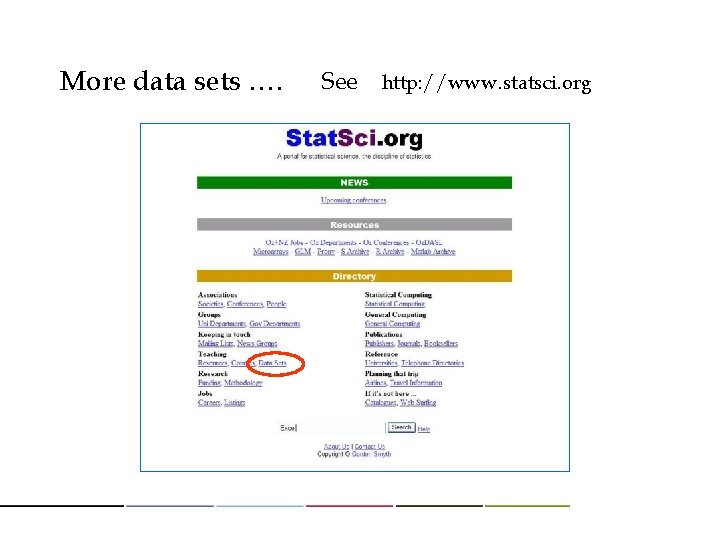
More data sets …. See http: //www. statsci. org

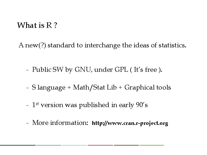
What is R ? A new(? ) standard to interchange the ideas of statistics. - Public SW by GNU, under GPL ( It’s free ). - S language + Math/Stat Lib + Graphical tools - 1 st version was published in early 90’s - More information: http: //www. cran. r-project. org

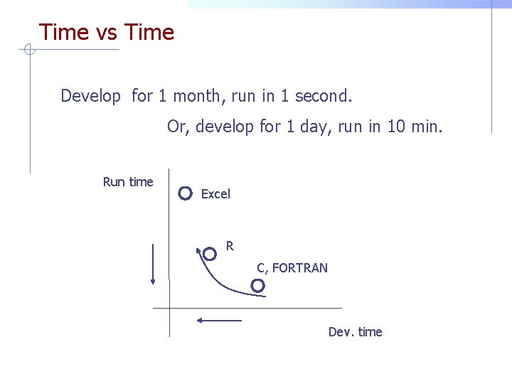
Time vs Time Develop for 1 month, run in 1 second. Or, develop for 1 day, run in 10 min. Run time Excel R C, FORTRAN Dev. time

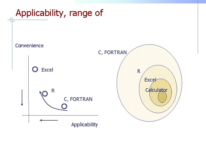
Applicability, range of Convenience C, FORTRAN Excel R Excel Calculator R C, FORTRAN Applicability

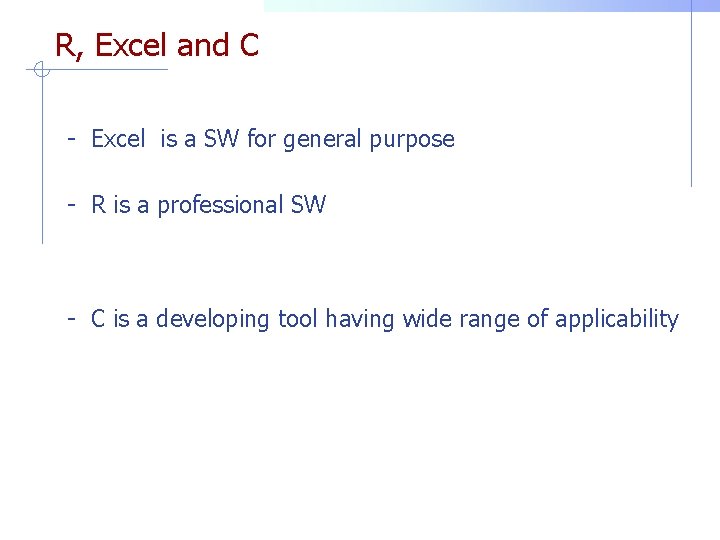
R, Excel and C - Excel is a SW for general purpose - R is a professional SW - C is a developing tool having wide range of applicability

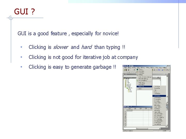
GUI ? GUI is a good feature , especially for novice! • Clicking is slower and hard than typing !! • Clicking is not good for iterative job at company • Clicking is easy to generate garbage !!

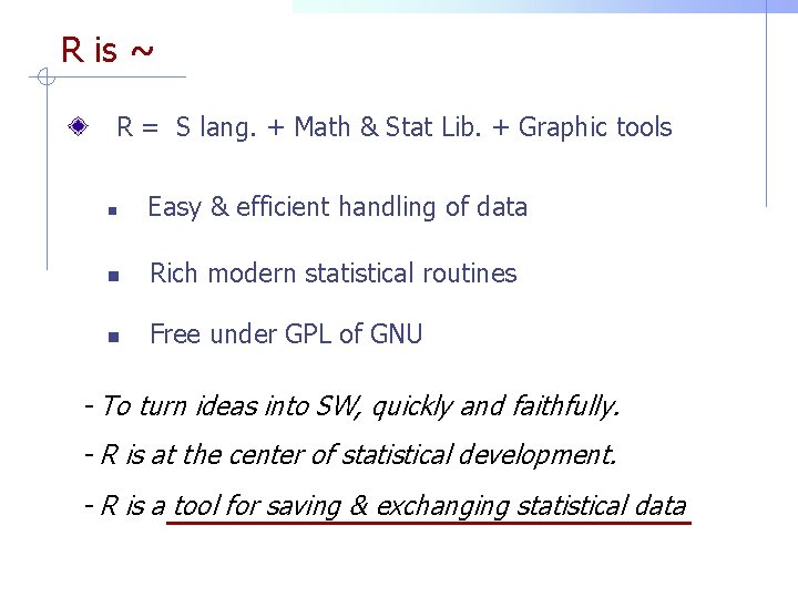
R is ~ R = S lang. + Math & Stat Lib. + Graphic tools n Easy & efficient handling of data n Rich modern statistical routines n Free under GPL of GNU - To turn ideas into SW, quickly and faithfully. - R is at the center of statistical development. - R is a tool for saving & exchanging statistical data

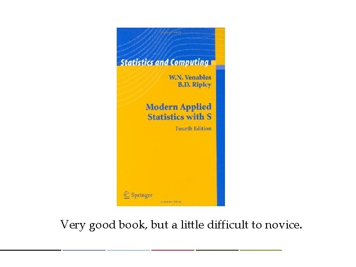
Very good book, but a little difficult to novice.

Easier alternatives

There are many easy books (try to find in amazon) and free tutorial guides in internet. Official free introductory guide: http: //cran. r-project. org/doc/manuals/R-intro. pdf

A free self study guide sites: http: //tryr. codeschool. com/ http: //www. sr. bham. ac. uk/~ajrs/R/index. html

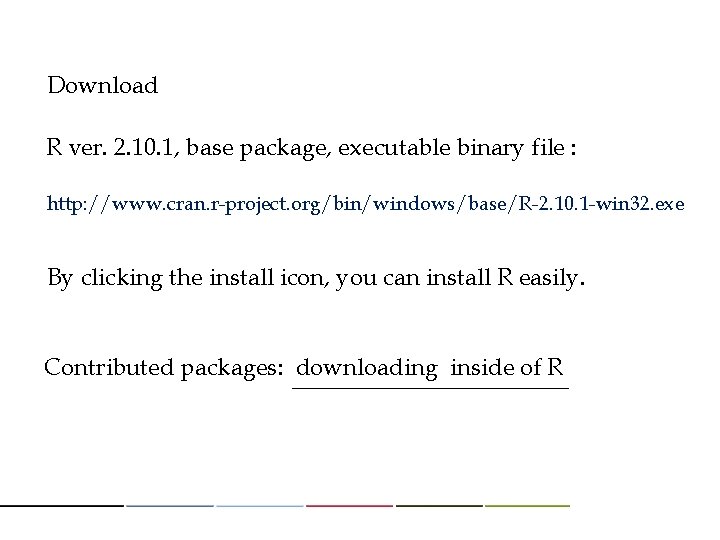
Download R ver. 2. 10. 1, base package, executable binary file : http: //www. cran. r-project. org/bin/windows/base/R-2. 10. 1 -win 32. exe By clicking the install icon, you can install R easily. Contributed packages: downloading inside of R

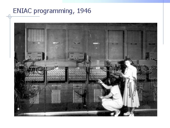
ENIAC programming, 1946

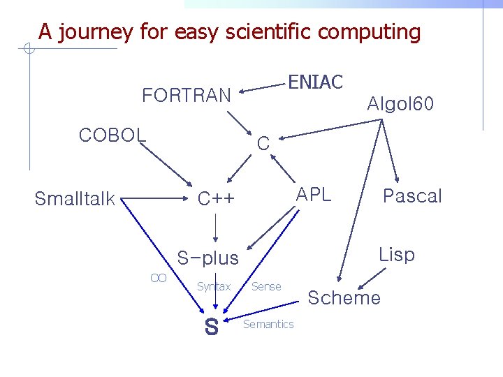
A journey for easy scientific computing ENIAC FORTRAN COBOL Algol 60 C Smalltalk APL C++ Lisp S-plus OO Pascal Syntax Sense S Semantics Scheme

Features of R 1. Vector Arithmetic (APL, S-plus) 2. Object Oriented property (Smalltalk, S-plus) 3. Lazy evaluation (S-plus) 4. (Nested) lexical scoping (Scheme, PASCAL)

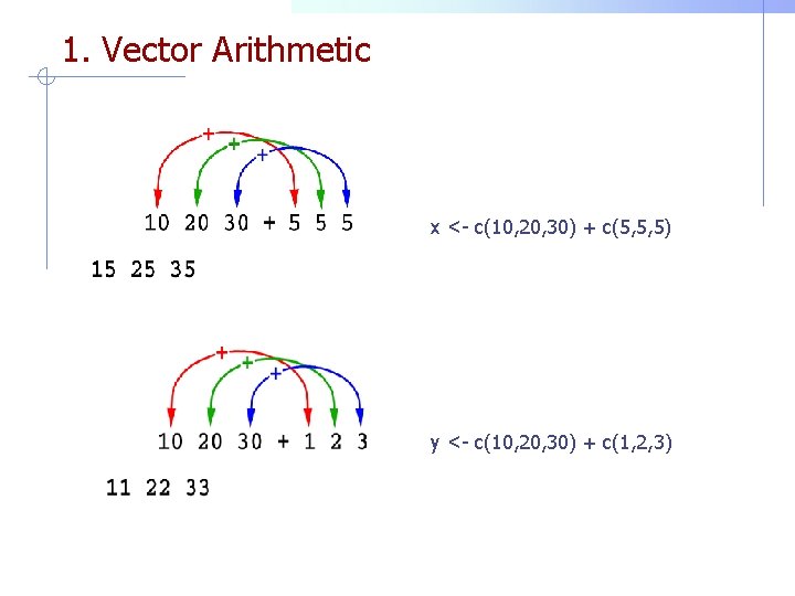
1. Vector Arithmetic x <- c(10, 20, 30) + c(5, 5, 5) y <- c(10, 20, 30) + c(1, 2, 3)

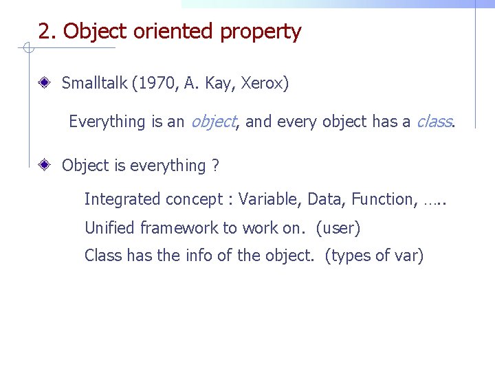
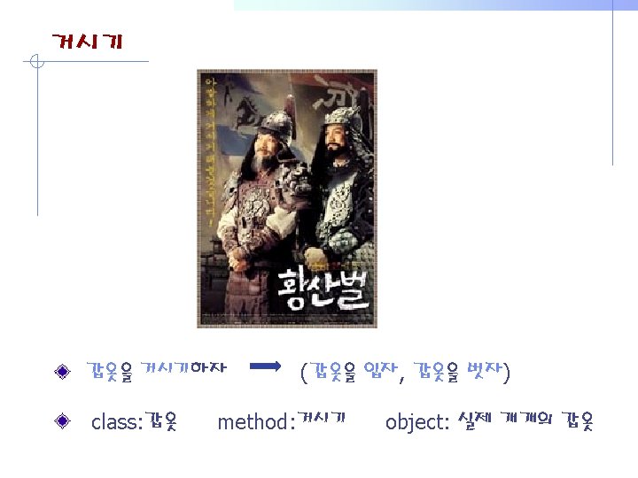
2. Object oriented property Smalltalk (1970, A. Kay, Xerox) Everything is an object, and every object has a class. Object is everything ? Integrated concept : Variable, Data, Function, …. . Unified framework to work on. (user) Class has the info of the object. (types of var)

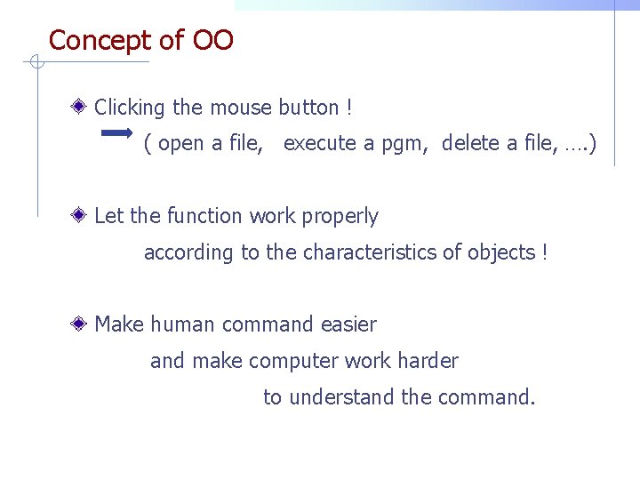
Concept of OO Clicking the mouse button ! ( open a file, execute a pgm, delete a file, …. ) Let the function work properly according to the characteristics of objects ! Make human command easier and make computer work harder to understand the command.

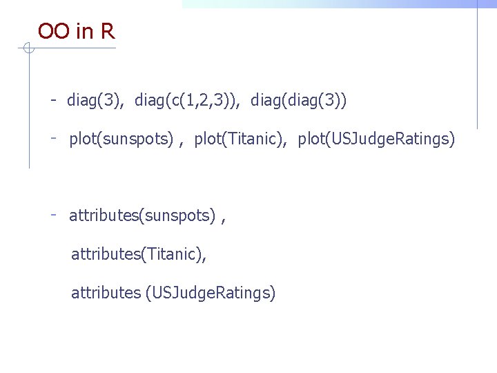
OO in R - diag(3), diag(c(1, 2, 3)), diag(3)) - plot(sunspots) , plot(Titanic), plot(USJudge. Ratings) - attributes(sunspots) , attributes(Titanic), attributes (USJudge. Ratings)

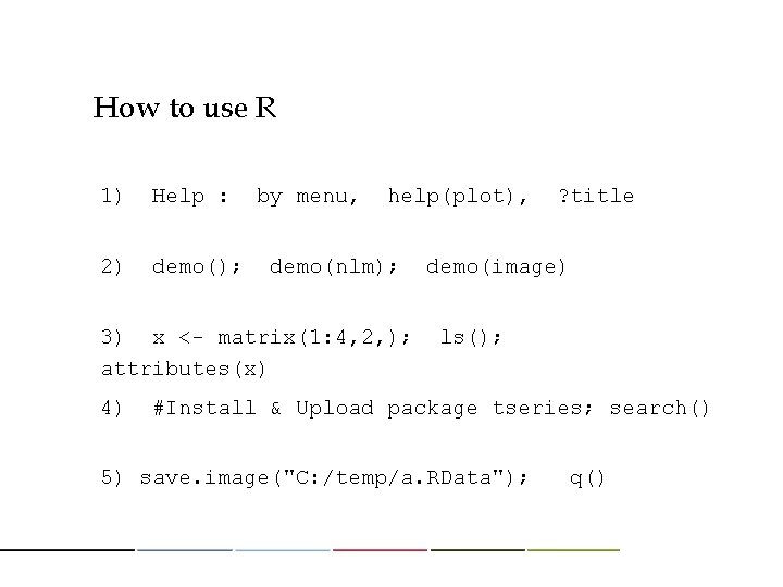
How to use R 1) Help : 2) demo(); by menu, help(plot), demo(nlm); 3) x <- matrix(1: 4, 2, ); attributes(x) 4) ? title demo(image) ls(); #Install & Upload package tseries; search() 5) save. image("C: /temp/a. RData"); q()

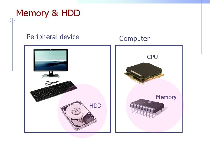
Memory & HDD Peripheral device Computer CPU Memory HDD

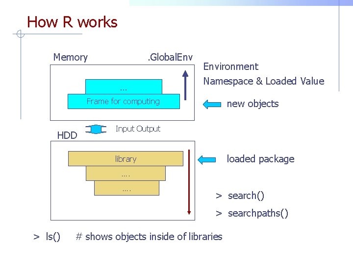
How R works Memory . Global. Env … Environment Namespace & Loaded Value Frame for computing HDD new objects Input Output loaded package library …. …. > search() > searchpaths() > ls() # shows objects inside of libraries

R data sets R has its own data sets for testing - data(); - Titanic; ? Titanic - plot(Titanic)

Data sets of SVV http: //www. aw. com/sharpe Get text file and excel file in your computer, and decompress. Make copies of text files under “C: temptext”

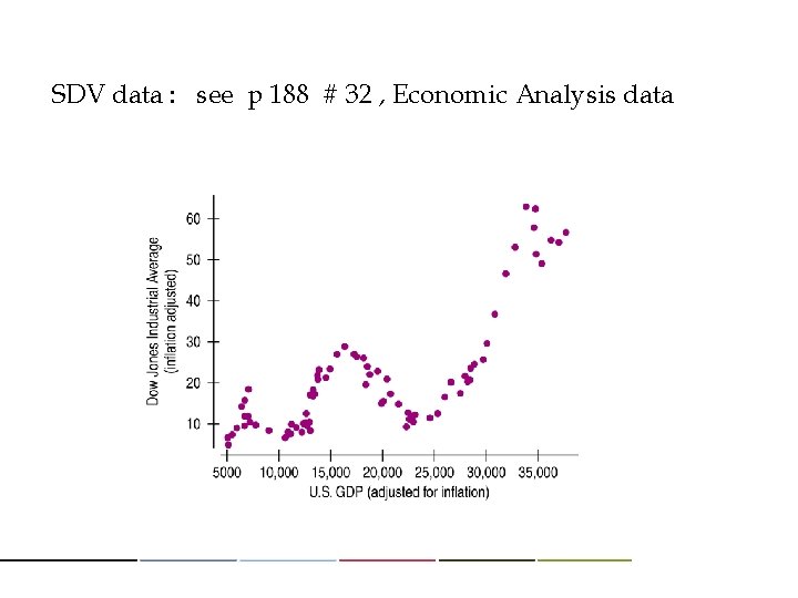
SDV data : see p 188 # 32 , Economic Analysis data

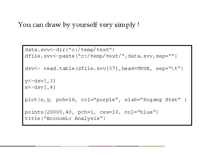
You can draw by yourself very simply ! data. svv<-dir("c: /temp/text") dfile. svv<-paste("c: /temp/text/", data. svv, sep="") dsv<- read. table(dfile. svv[37], head=TRUE, sep="t") y<-dsv[, 3] x<-dsv[, 4] plot(x, y, pch=16, col="purple", xlab="Sogang Stat" ) points(20000, 40, pch=1, cex=10, col="blue") title("Economic Analysis")

Install & load packages Memory Server Load Internet HDD Install

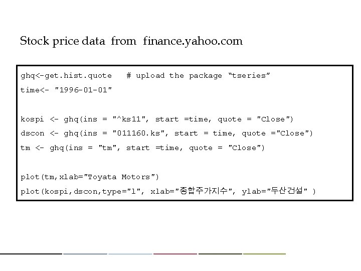
Stock price data from finance. yahoo. com ghq<-get. hist. quote # upload the package “tseries” time<- "1996 -01 -01" kospi <- ghq(ins = "^ks 11", start =time, quote = "Close") dscon <- ghq(ins = "011160. ks", start = time, quote ="Close") tm <- ghq(ins = "tm", start =time, quote = "Close") plot(tm, xlab="Toyata Motors") plot(kospi, dscon, type="l", xlab="종합주가지수", ylab="두산건설" )

Hanoi Tower By simple programming, graphical implementation of Hanoi tower is possible in R. The code & program were loaded to cyber campus. - hanoi(4) - hanoi(14)

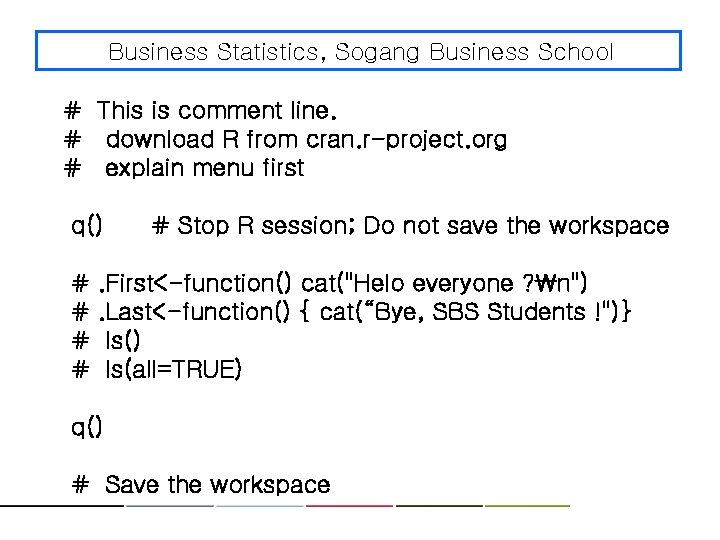
Business Statistics, Sogang Business School # This is comment line. # download R from cran. r-project. org # explain menu first q() # # # Stop R session; Do not save the workspace . First<-function() cat("Helo everyone ? n"). Last<-function() { cat(“Bye, SBS Students !")} ls() ls(all=TRUE) q() # Save the workspace

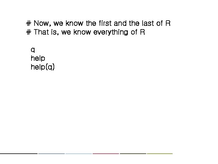
# Now, we know the first and the last of R # That is, we know everything of R q help(q)

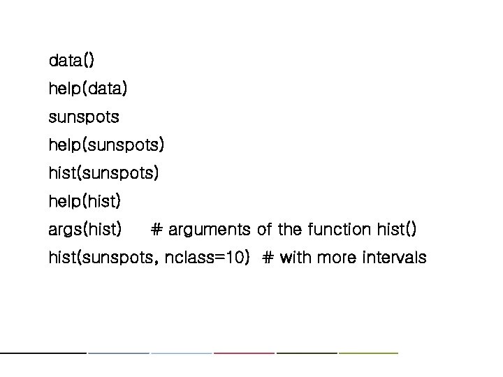
data() help(data) sunspots help(sunspots) hist(sunspots) help(hist) args(hist) # arguments of the function hist() hist(sunspots, nclass=10) # with more intervals

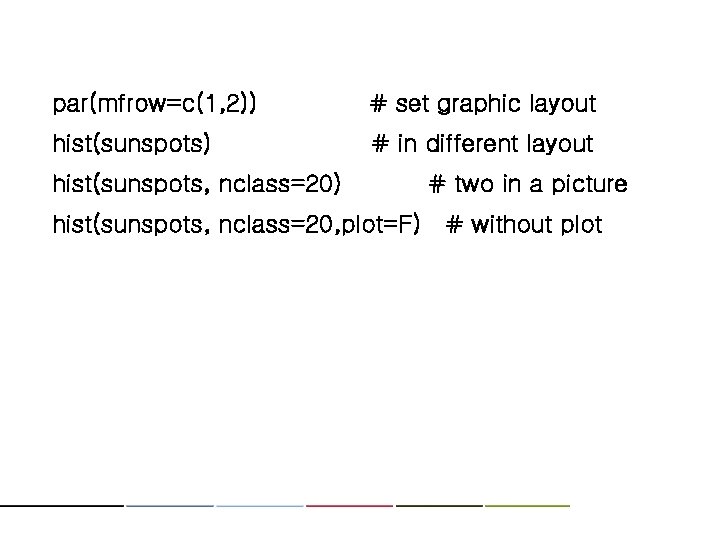
par(mfrow=c(1, 2)) # set graphic layout hist(sunspots) # in different layout hist(sunspots, nclass=20) # two in a picture hist(sunspots, nclass=20, plot=F) # without plot

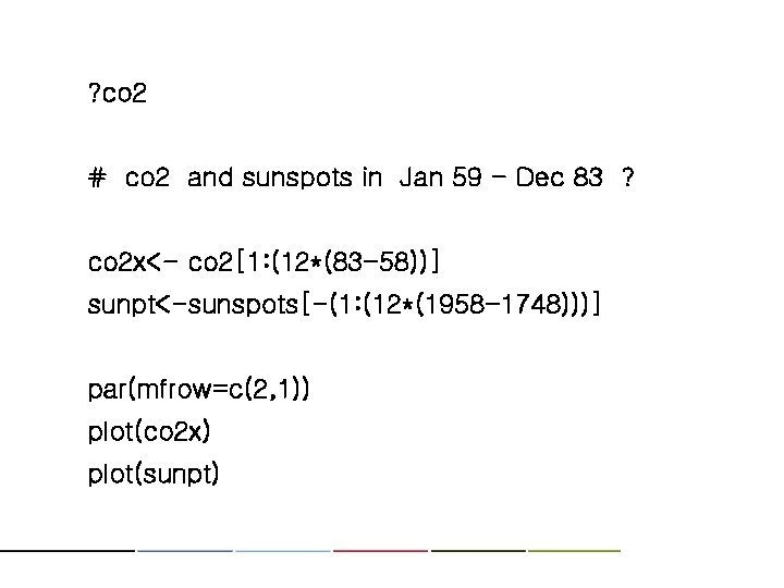
? co 2 # co 2 and sunspots in Jan 59 - Dec 83 ? co 2 x<- co 2[1: (12*(83 -58))] sunpt<-sunspots[-(1: (12*(1958 -1748)))] par(mfrow=c(2, 1)) plot(co 2 x) plot(sunpt)

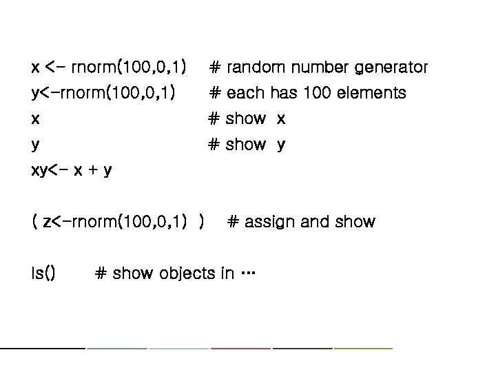
x <- rnorm(100, 0, 1) # random number generator y<-rnorm(100, 0, 1) # each has 100 elements x # show x y # show y xy<- x + y ( z<-rnorm(100, 0, 1) ) ls() # assign and show # show objects in …

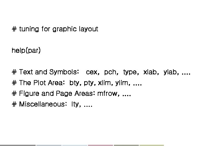
# tuning for graphic layout help(par) # Text and Symbols: cex, pch, type, xlab, ylab, . . # The Plot Area: bty, pty, xlim, ylim, . . # Figure and Page Areas: mfrow, . . # Miscellaneous: lty, . .

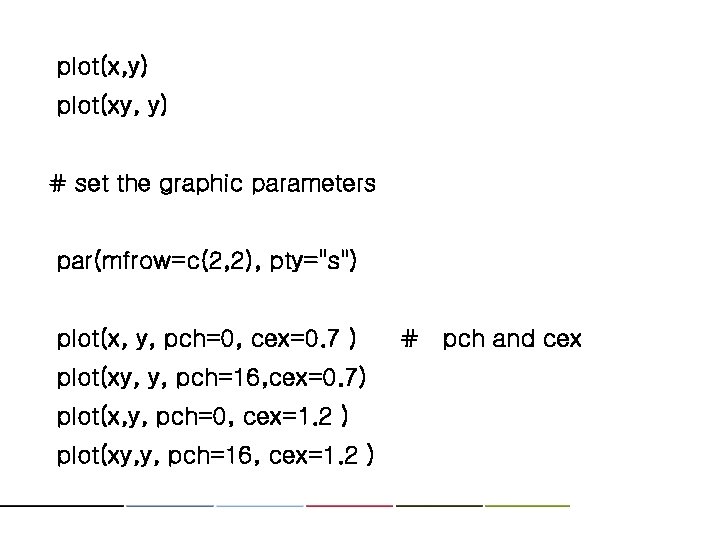
plot(x, y) plot(xy, y) # set the graphic parameters par(mfrow=c(2, 2), pty="s") plot(x, y, pch=0, cex=0. 7 ) plot(xy, y, pch=16, cex=0. 7) plot(x, y, pch=0, cex=1. 2 ) plot(xy, y, pch=16, cex=1. 2 ) # pch and cex

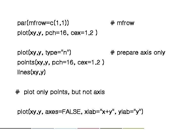
par(mfrow=c(1, 1)) # mfrow plot(xy, y, pch=16, cex=1. 2 ) plot(xy, y, type="n") # prepare axis only points(xy, y, pch=16, cex=1. 2 ) lines(xy, y) # plot only points, but not axis plot(xy, y, axes=FALSE, xlab="x+y", ylab="y")

cbind(x, y, xy) # column binding y[y>0] xy[y>0] cbind(x, y, xy) [y>0] plot(xy, y, type="n", xlab="x+y", ylab="y" ) # axis only points(xy[y>0], pch=16, cex=0. 6 ) # for y>0 points(xy[y<=0], pch=1, cex=0. 8 ) # y <= 0

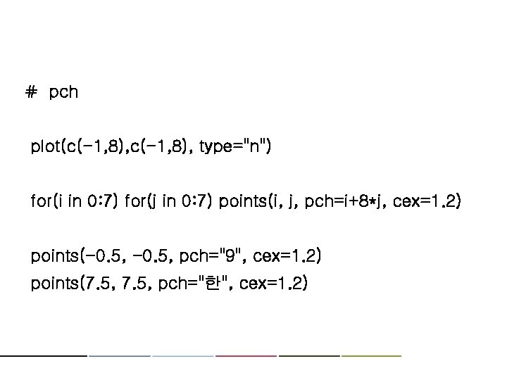
# pch plot(c(-1, 8), type="n") for(i in 0: 7) for(j in 0: 7) points(i, j, pch=i+8*j, cex=1. 2) points(-0. 5, pch="9", cex=1. 2) points(7. 5, pch="한", cex=1. 2)

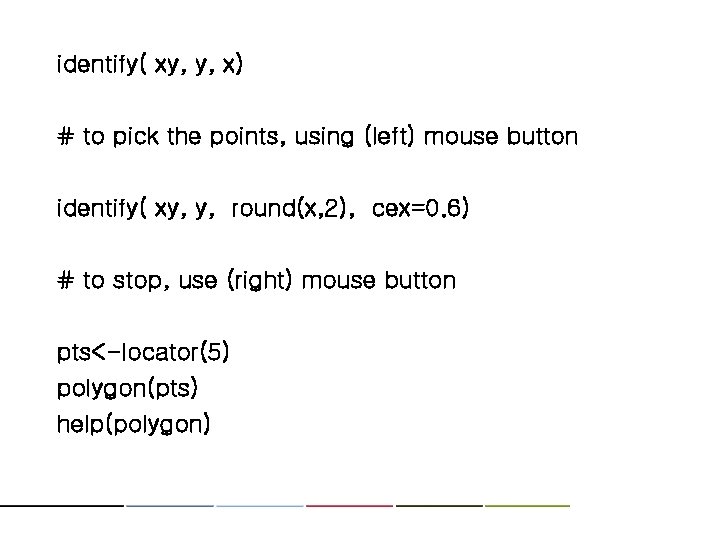
identify( xy, y, x) # to pick the points, using (left) mouse button identify( xy, y, round(x, 2), cex=0. 6) # to stop, use (right) mouse button pts<-locator(5) polygon(pts) help(polygon)

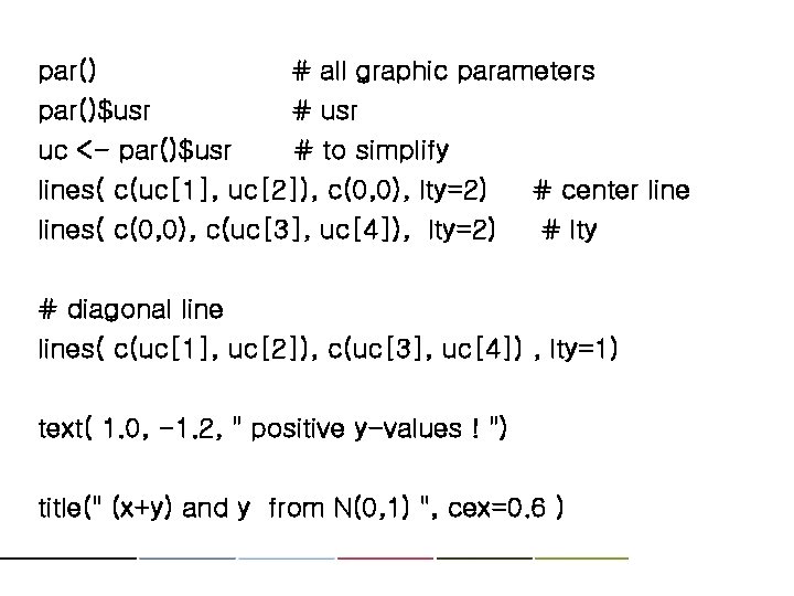
par()$usr uc <- par()$usr # all graphic parameters # usr # to simplify lines( c(uc[1], uc[2]), c(0, 0), lty=2) lines( c(0, 0), c(uc[3], uc[4]), lty=2) # center line # lty # diagonal lines( c(uc[1], uc[2]), c(uc[3], uc[4]) , lty=1) text( 1. 0, -1. 2, " positive y-values ! ") title(" (x+y) and y from N(0, 1) ", cex=0. 6 )

help(USJudge. Ratings) USJudge. Ratings pairs(USJudge. Ratings) pairs(USJudge. Ratings[1: 5])

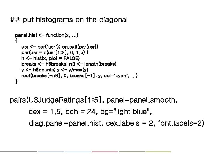
## put histograms on the diagonal panel. hist <- function(x, . . . ) { usr <- par("usr"); on. exit(par(usr)) par(usr = c(usr[1: 2], 0, 1. 5) ) h <- hist(x, plot = FALSE) breaks <- h$breaks; n. B <- length(breaks) y <- h$counts; y <- y/max(y) rect(breaks[-n. B], 0, breaks[-1], y, col="cyan", . . . ) } pairs(USJudge. Ratings[1: 5], panel=panel. smooth, cex = 1. 5, pch = 24, bg="light blue", diag. panel=panel. hist, cex. labels = 2, font. labels=2)

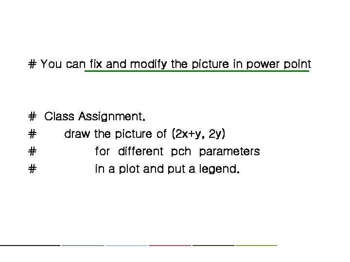
# You can fix and modify the picture in power point # Class Assignment. # draw the picture of (2 x+y, 2 y) # for different pch parameters # in a plot and put a legend.

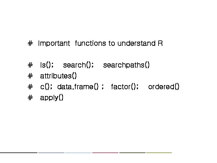
# Important functions to understand R # ls(); searchpaths() # attributes() # c(); data. frame() ; factor(); # apply() ordered()

Thank you !!