Statistical Software Programming 1 STAT 6360 Statistical Software

Statistical Software Programming 1

STAT 6360 –Statistical Software Programming Modifying and Combining Datasets • For most tasks we need to work with multiple datasets to accomplish our goal. Therefore we need to know how to combine datasets in various ways. • In addition, datasets created previously or with a PROC may need to be modified. How do we access the dataset again to create new variables, modify data, select observations, etc. ? 2

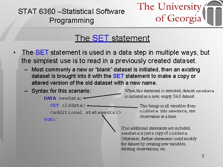
STAT 6360 –Statistical Software Programming The SET statement • The SET statement is used in a data step in multiple ways, but the simplest use is to read in a previously created dataset. – Most commonly a new or “blank” dataset is initiated, then an existing dataset is brought into it with the SET statement to make a copy or altered version of the old dataset with a new name. When this statement is executed, dataset newdata – Syntax for this scenario: is initiated as a new, empty SAS dataset. DATA newdata; SET olddata; This brings in all variables from olddata into newdata, one <additional statements; > observation at a time. RUN; ` If no additional statements are included, newdata is just a copy of olddata. Otherwise, further statements could modify the dataset by creating new variables, deleting observations, etc. 3

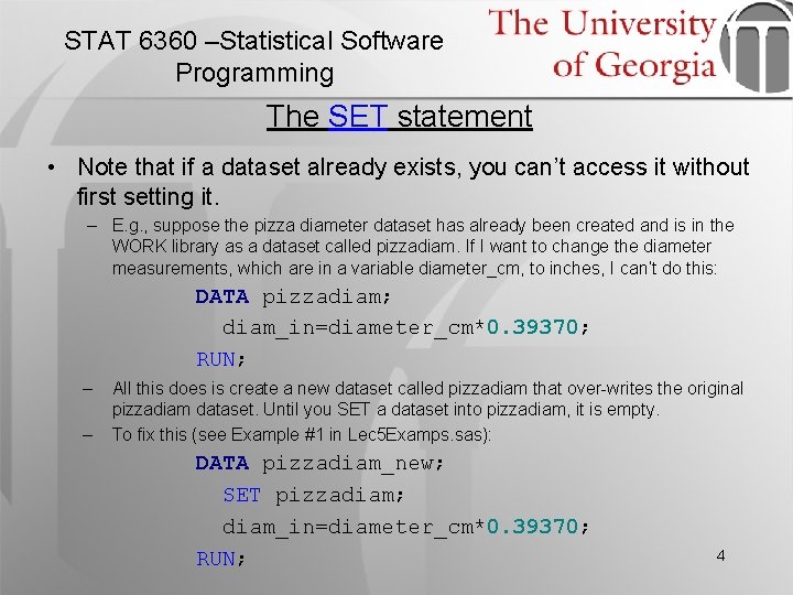
STAT 6360 –Statistical Software Programming The SET statement • Note that if a dataset already exists, you can’t access it without first setting it. – E. g. , suppose the pizza diameter dataset has already been created and is in the WORK library as a dataset called pizzadiam. If I want to change the diameter measurements, which are in a variable diameter_cm, to inches, I can’t do this: DATA pizzadiam; diam_in=diameter_cm*0. 39370; RUN; – – All this does is create a new dataset called pizzadiam that over-writes the original pizzadiam dataset. Until you SET a dataset into pizzadiam, it is empty. To fix this (see Example #1 in Lec 5 Examps. sas): DATA pizzadiam_new; SET pizzadiam; diam_in=diameter_cm*0. 39370; RUN; 4

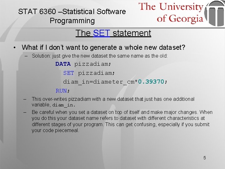
STAT 6360 –Statistical Software Programming The SET statement • What if I don’t want to generate a whole new dataset? – Solution: just give the new dataset the same name as the old: DATA pizzadiam; SET pizzadiam; diam_in=diameter_cm*0. 39370; RUN; – This over-writes pizzadiam with a new dataset that just has one additional variable, diam_in. – Be careful when you set a dataset on top of itself and make major changes. When you do this your dataset name refers to dataset with different characteristics at different stages of your program. This can get confusing, especially if you submit your code piecemeal. 5

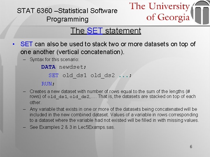
STAT 6360 –Statistical Software Programming The SET statement • SET can also be used to stack two or more datasets on top of one another (vertical concatenation). – Syntax for this scenario: DATA newdset; SET old_ds 1 old_ds 2. . . ; RUN; – Creates a new dataset with number of rows equal to the sum of the lengths (# rows) of old_ds 1, old_ds 2, …. That is, the datasets are stacked on top of each other. – Any variable that exists in one or more of the datasets being concatenated will be included in the new combined dataset. Values of a variable in rows corresponding to a dataset where the variable had not existed will be filled in with missing values. – See Examples 2 & 3 in Lec 5 Examps. sas. 6

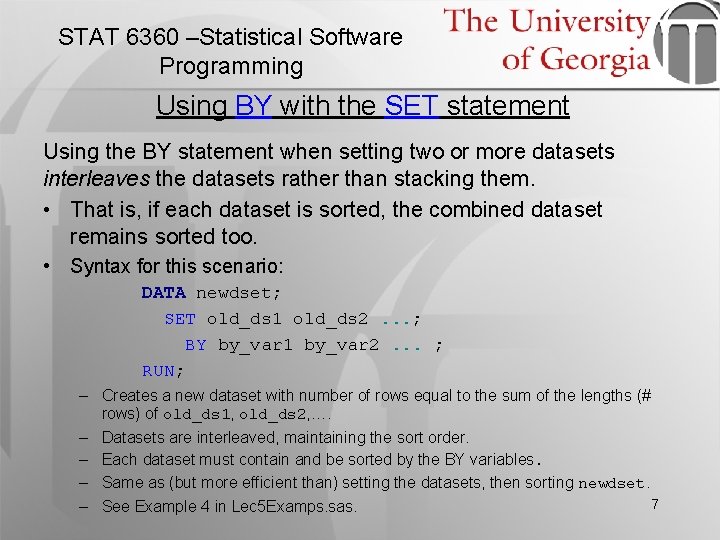
STAT 6360 –Statistical Software Programming Using BY with the SET statement Using the BY statement when setting two or more datasets interleaves the datasets rather than stacking them. • That is, if each dataset is sorted, the combined dataset remains sorted too. • Syntax for this scenario: DATA newdset; SET old_ds 1 old_ds 2. . . ; BY by_var 1 by_var 2. . . ; RUN; – Creates a new dataset with number of rows equal to the sum of the lengths (# rows) of old_ds 1, old_ds 2, …. – Datasets are interleaved, maintaining the sort order. – Each dataset must contain and be sorted by the BY variables. – Same as (but more efficient than) setting the datasets, then sorting newdset. 7 – See Example 4 in Lec 5 Examps. sas.

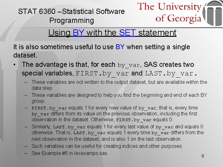
STAT 6360 –Statistical Software Programming Using BY with the SET statement It is also sometimes useful to use BY when setting a single dataset. • The advantage is that, for each by_var, SAS creates two special variables, FIRST. by_var and LAST. by_var. – These variables are not written to the output dataset, but are available within the data step. – These variables are designed to help you find the beginning and end of each BY group. – FIRST. by_var equals 1 for every new value of by_var; that is, every time by_var differs from its value on the previous observation, including the first observation in the dataset. Otherwise, FIRST. by_var equals 0. – Similarly, LAST. by_var equals 1 for every last value of by_var and equals 0 otherwise. That is, LAST. by_var equals 1 every time by_var differs from the next observation in the dataset, and is also 1 on the last observation. – Such variables can be useful for creating indices and other purposes. – See Example #5 in lecexamps. sas. 8

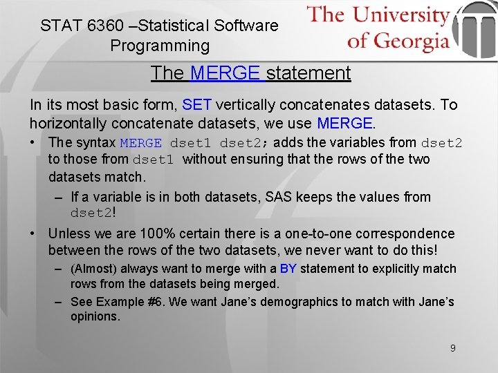
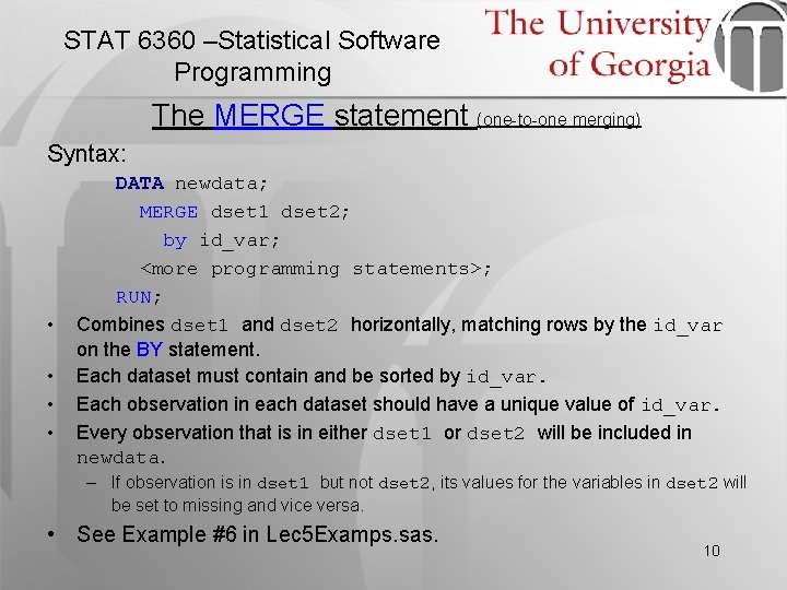
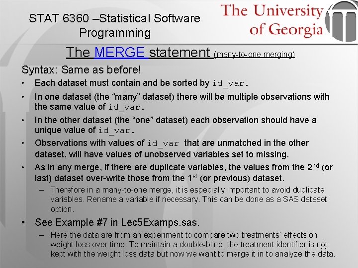
STAT 6360 –Statistical Software Programming The MERGE statement In its most basic form, SET vertically concatenates datasets. To horizontally concatenate datasets, we use MERGE. • The syntax MERGE dset 1 dset 2; adds the variables from dset 2 to those from dset 1 without ensuring that the rows of the two datasets match. – If a variable is in both datasets, SAS keeps the values from dset 2! • Unless we are 100% certain there is a one-to-one correspondence between the rows of the two datasets, we never want to do this! – (Almost) always want to merge with a BY statement to explicitly match rows from the datasets being merged. – See Example #6. We want Jane’s demographics to match with Jane’s opinions. 9

STAT 6360 –Statistical Software Programming The MERGE statement (one-to-one merging) Syntax: • • DATA newdata; MERGE dset 1 dset 2; by id_var; <more programming statements>; RUN; Combines dset 1 and dset 2 horizontally, matching rows by the id_var on the BY statement. Each dataset must contain and be sorted by id_var. Each observation in each dataset should have a unique value of id_var. Every observation that is in either dset 1 or dset 2 will be included in newdata. – If observation is in dset 1 but not dset 2, its values for the variables in dset 2 will be set to missing and vice versa. • See Example #6 in Lec 5 Examps. sas. 10

STAT 6360 –Statistical Software Programming The MERGE statement (many-to-one merging) Syntax: Same as before! • • Each dataset must contain and be sorted by id_var. • In the other dataset (the “one” dataset) each observation should have a unique value of id_var. Observations with values of id_var that are unmatched in the other dataset, will have values of unobserved variables set to missing. As in any merge, if there are duplicate variables, the values from the 2 nd (or last) dataset over-write those from the 1 st (or previous) dataset. • • In one dataset (the “many” dataset) there will be multiple observations with the same value of id_var. – Therefore in a many-to-one merge, it is especially important to avoid duplicate variables. Rename a variable if necessary. This can be done as a SAS dataset option. • See Example #7 in Lec 5 Examps. sas. – Here the data are from an experiment to compare two treatments’ effects on weight loss over time. To maintain a double-blind, the treatment identifier is not 11 kept with the weight loss data but now we want to merge it in to analyze the data.

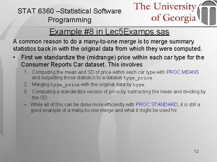
STAT 6360 –Statistical Software Programming Example #8 in Lec 5 Examps. sas A common reason to do a many-to-one merge is to merge summary statistics back in with the original data from which they were computed. • First we standardize the (midrange) price within each car type for the Consumer Reports Car dataset. This involves 1. Computing the mean and SD of price within each car type with PROC MEANS and outputting those statistics to a dataset type_price. 2. Merging type_price with the original data by type. 3. Computing a standardize version of price by subtracting the mean and dividing by the SD. – While all of this can be done more efficiently with PROC STANDARD, it is still a good example of a many-to-one merge and what it might be used for. 12

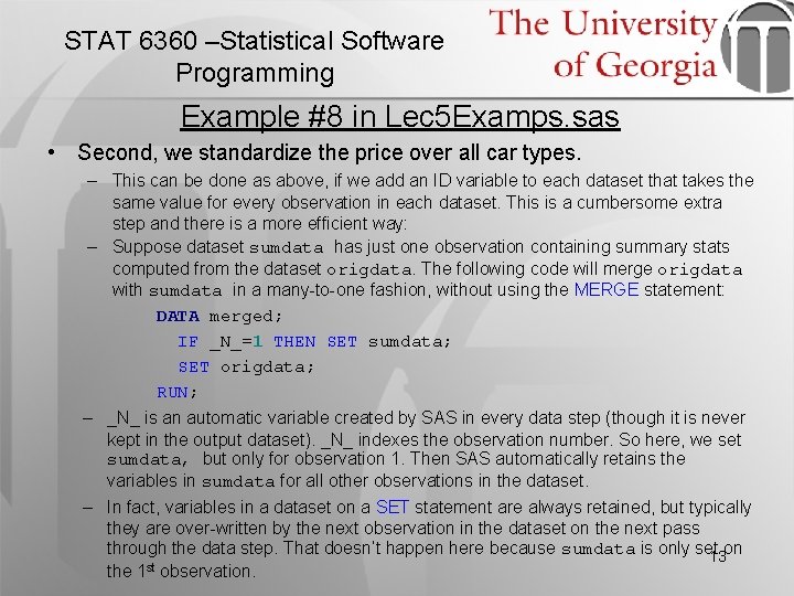
STAT 6360 –Statistical Software Programming Example #8 in Lec 5 Examps. sas • Second, we standardize the price over all car types. – This can be done as above, if we add an ID variable to each dataset that takes the same value for every observation in each dataset. This is a cumbersome extra step and there is a more efficient way: – Suppose dataset sumdata has just one observation containing summary stats computed from the dataset origdata. The following code will merge origdata with sumdata in a many-to-one fashion, without using the MERGE statement: DATA merged; IF _N_=1 THEN SET sumdata; SET origdata; RUN; – _N_ is an automatic variable created by SAS in every data step (though it is never kept in the output dataset). _N_ indexes the observation number. So here, we set sumdata, but only for observation 1. Then SAS automatically retains the variables in sumdata for all other observations in the dataset. – In fact, variables in a dataset on a SET statement are always retained, but typically they are over-written by the next observation in the dataset on the next pass through the data step. That doesn’t happen here because sumdata is only set on 13 the 1 st observation.

STAT 6360 –Statistical Software Programming The OUTPUT Statement (in a data step) We have used OUTPUT in PROC MEANS, and there are similar statements in several other PROCs. However, there is also an OUTPUT statement in a data step that is worth knowing. • A data step processes each observation one at a time and, with the data from that observation, executes each line, one at a time using a temporary program data vector (PDV). • When it reaches the end of the data step (e. g. , the RUN statement), the data from the PDV is output to the dataset being created. – This is an implicit execution of an OUTPUT statement that SAS does automatically, every time through the dataset. 14

STAT 6360 –Statistical Software Programming The OUTPUT Statement (in a data step) • The OUTPUT statement allows you to control when the data from the PDV are output. This allows you to – Create multiple observations in the output dataset from each observation in the data being processed. – Create more than one dataset at a time. – Create an output dataset that is smaller than (a subset of, or processed version of) the data being read in (via INPUT, or SET, say). – Create a dataset without reading in any data at all. • If an OUTPUT statement is used, it cancels the implicit output at the end of the data step. 15

STAT 6360 –Statistical Software Programming The OUTPUT Statement - Examples Example #9 – Generating the Explanatory Variables from an Experimental Design • Consider a two-way layout with factors A and B, with 3 and 2 levels, respectively, with 4 replicates/treatment. • Example #9 generates factors A, B and indicator variables for each level of each factor and for each treatment and outputs them to a dataset called two_way. • No data are read in; instead, multiple observations are created by placing OUTPUT inside 3 nested DO loops. – It is important that OUTPUT appear after the variables have been created. – To see what happens to variables created after the OUTPUT statement, uncomment the line after the OUTPUT statement and re-run the program. The variable X isn’t assigned until after the observation has been written to the output dataset. 16

STAT 6360 –Statistical Software Programming The OUTPUT Statement - Examples Example #10 – Transposing Variables to Observations within a Subject. • The dataset bodymeas first appeared in lec 3 examps. sas. It contains body measurements (height, weight, sitting height) measures at 0, 6 and 12 months from the beginning of a study. • Here, we reorganize the data so that each subject has three observations, one per measurement occasion. • Again, using OUTPUT within a DO loop does the trick. • Notice that the variable indexing the DO loop is set to increment by 6, over-riding the default increment of 1. • Also note the use of the KEEP statement. There is a similar statement called DROP. These statements allow you to restrict which variables are retained in the output dataset. Use one 17 or the other, not both.

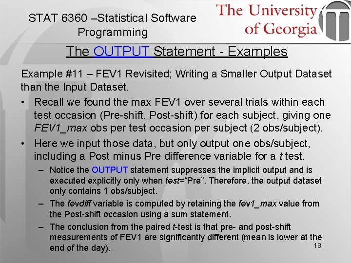
STAT 6360 –Statistical Software Programming The OUTPUT Statement - Examples Example #11 – FEV 1 Revisited; Writing a Smaller Output Dataset than the Input Dataset. • Recall we found the max FEV 1 over several trials within each test occasion (Pre-shift, Post-shift) for each subject, giving one FEV 1_max obs per test occasion per subject (2 obs/subject). • Here we input those data, but only output one obs/subject, including a Post minus Pre difference variable for a t test. – Notice the OUTPUT statement suppresses the implicit output and is executed explicitly only when test=“Pre”. Therefore, the output dataset only contains 1 obs/subject. – The fevdiff variable is computed by retaining the fev 1_max value from the Post-shift occasion using a sum statement. – The conclusion from the paired t-test is that pre- and post-shift measurements of FEV 1 are significantly different (mean is lower at the 18 end of the day).

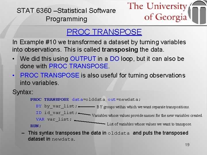
STAT 6360 –Statistical Software Programming PROC TRANSPOSE In Example #10 we transformed a dataset by turning variables into observations. This is called transposing the data. • We did this using OUTPUT in a DO loop, but it can also be done with PROC TRANSPOSE. • PROC TRANSPOSE is also useful for turning observations into variables. Syntax: PROC TRANSPOSE data=olddata out=newdata; BY by_var_list; BY groups within which we want separate transpositions. ID id_var_list; Variables whose values provide names for the new variables created. VAR var_list; List of variables whose values we want to transpose. RUN; – This syntax transposes the data in olddata and puts the transposed dataset in newdata. 19

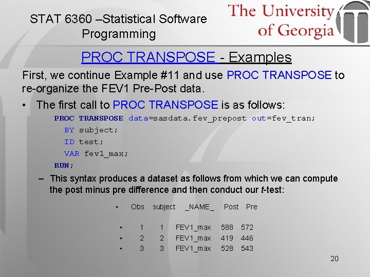
STAT 6360 –Statistical Software Programming PROC TRANSPOSE - Examples First, we continue Example #11 and use PROC TRANSPOSE to re-organize the FEV 1 Pre-Post data. • The first call to PROC TRANSPOSE is as follows: PROC TRANSPOSE data=sasdata. fev_prepost out=fev_tran; BY subject; ID test; VAR fev 1_max; RUN; – This syntax produces a dataset as follows from which we can compute the post minus pre difference and then conduct our t-test: • Obs • • • 1 2 3 subject 1 2 3 _NAME_ FEV 1_max Post 588 419 528 Pre 572 446 543 20

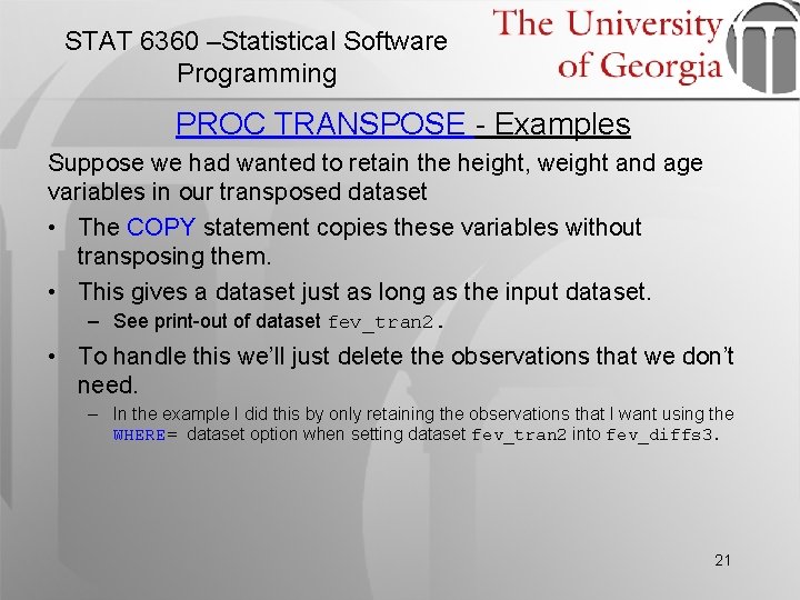
STAT 6360 –Statistical Software Programming PROC TRANSPOSE - Examples Suppose we had wanted to retain the height, weight and age variables in our transposed dataset • The COPY statement copies these variables without transposing them. • This gives a dataset just as long as the input dataset. – See print-out of dataset fev_tran 2. • To handle this we’ll just delete the observations that we don’t need. – In the example I did this by only retaining the observations that I want using the WHERE= dataset option when setting dataset fev_tran 2 into fev_diffs 3. 21

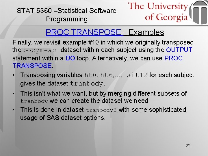
STAT 6360 –Statistical Software Programming PROC TRANSPOSE - Examples Finally, we revisit example #10 in which we originally transposed the bodymeas dataset within each subject using the OUTPUT statement within a DO loop. Alternatively, we can use PROC TRANSPOSE. • Transposing variables ht 0, ht 6, …, sit 12 for each subject gives the dataset tranbody. • This isn’t what we want, but by merging different subsets of tranbody we can create the dataset we need. • This is done in dataset tranbody 2 with some sophisticated usage of SAS dataset options. 22

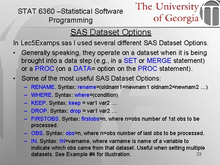
STAT 6360 –Statistical Software Programming SAS Dataset Options In Lec 5 Examps. sas I used several different SAS Dataset Options. • Generally speaking, they operate on a dataset when it is being brought into a data step (e. g. , in a SET or MERGE statement) or a PROC (on a DATA= option on the PROC statement). • Some of the most useful SAS Dataset Options: – – – RENAME. Syntax: rename=(oldnam 1=newnam 1 oldnam 2=newnam 2 …) WHERE. Syntax: where=(condition) KEEP. Syntax: keep = var 1 var 2 … DROP. Syntax: drop = var 1 var 2 … FIRSTOBS. Syntax: firstobs=n, where n=obs number of 1 st obs to be processed. – OBS. Syntax: obs=n, where n=obs number of last obs to be processed. – IN. Syntax: IN=varname, where varname is name of a variable to indicate which obs came from that dataset. Useful when setting multiple 23 datasets. See Example #4 for illustration.

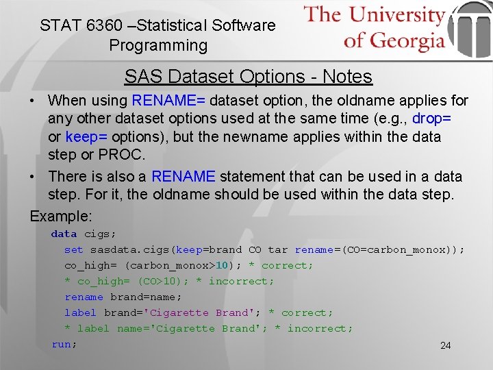
STAT 6360 –Statistical Software Programming SAS Dataset Options - Notes • When using RENAME= dataset option, the oldname applies for any other dataset options used at the same time (e. g. , drop= or keep= options), but the newname applies within the data step or PROC. • There is also a RENAME statement that can be used in a data step. For it, the oldname should be used within the data step. Example: data cigs; set sasdata. cigs(keep=brand CO tar rename=(CO=carbon_monox)); co_high= (carbon_monox>10); * correct; * co_high= (CO>10); * incorrect; rename brand=name; label brand='Cigarette Brand'; * correct; * label name='Cigarette Brand'; * incorrect; run; 24