Statistical Significance Test 1 Why Statistical Significance Test

Statistical Significance Test 1

Why Statistical Significance Test • • Suppose we have developed an EC algorithm A We want to compare with another EC algorithm B Both algorithms are stochastic How can we be sure that A is better than B? • Assume we run A and B once, and get the results x and y, respectively. • If x < y (minimisation), is it because A is better than B, or just because of randomness? 2

Why Statistical Significance Test • Treat a stochastic algorithm as a random number generator, and its output follows some distribution • The random output depends on the algorithm and random seed • Collect samples: run algorithms many times independently (using different random seeds) • Carry out statistical significance tests based on the collected samples 3

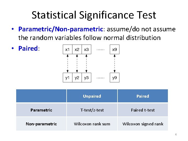
Statistical Significance Test • Parametric/Non-parametric: assume/do not assume the random variables follow normal distribution • Paired: Unpaired Parametric T-test/z-test Paired t-test Non-parametric Wilcoxon rank sum Wilcoxon signed rank 4

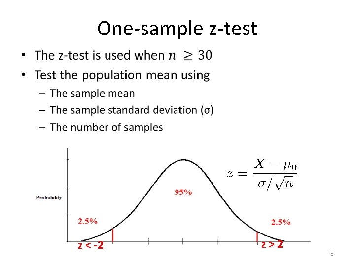
One-sample z-test • z < -2 z>2 5

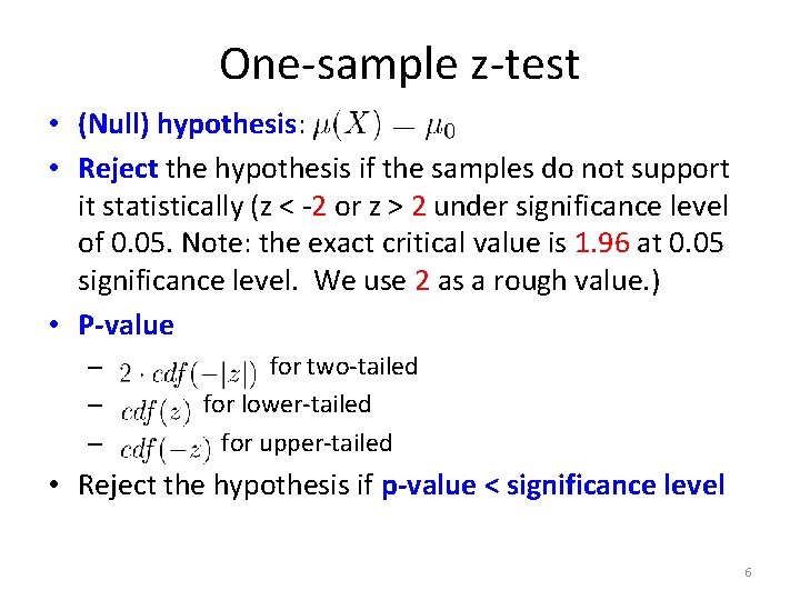
One-sample z-test • (Null) hypothesis: • Reject the hypothesis if the samples do not support it statistically (z < -2 or z > 2 under significance level of 0. 05. Note: the exact critical value is 1. 96 at 0. 05 significance level. We use 2 as a rough value. ) • P-value – for two-tailed – for lower-tailed – for upper-tailed • Reject the hypothesis if p-value < significance level 6

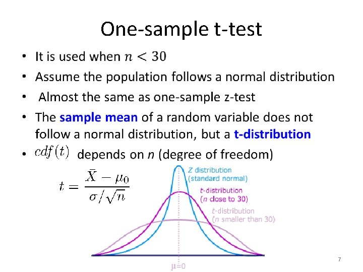
One-sample t-test • 7

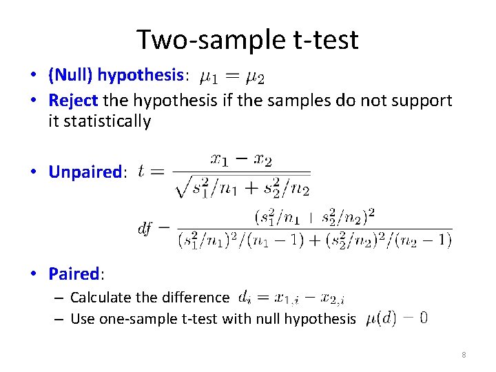
Two-sample t-test • (Null) hypothesis: • Reject the hypothesis if the samples do not support it statistically • Unpaired: • Paired: – Calculate the difference – Use one-sample t-test with null hypothesis 8

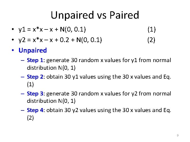
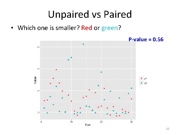
Unpaired vs Paired • y 1 = x*x – x + N(0, 0. 1) (1) • y 2 = x*x – x + 0. 2 + N(0, 0. 1) (2) • Unpaired – Step 1: generate 30 random x values for y 1 from normal distribution N(0, 1) – Step 2: obtain 30 y 1 values using the 30 x values and Eq. (1) – Step 3: generate 30 random x values for y 2 from normal distribution N(0, 1) – Step 4: obtain 30 y 2 values using the 30 x values and Eq. (2) 9

Unpaired vs Paired • Which one is smaller? Red or green? P-value = 0. 56 10

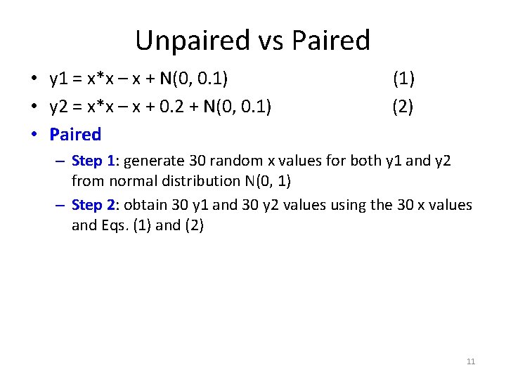
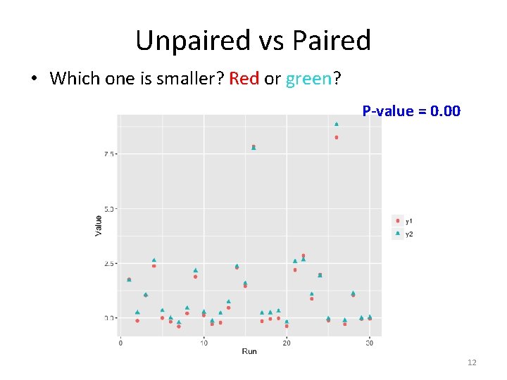
Unpaired vs Paired • y 1 = x*x – x + N(0, 0. 1) (1) • y 2 = x*x – x + 0. 2 + N(0, 0. 1) (2) • Paired – Step 1: generate 30 random x values for both y 1 and y 2 from normal distribution N(0, 1) – Step 2: obtain 30 y 1 and 30 y 2 values using the 30 x values and Eqs. (1) and (2) 11

Unpaired vs Paired • Which one is smaller? Red or green? P-value = 0. 00 12

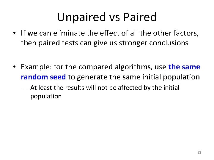
Unpaired vs Paired • If we can eliminate the effect of all the other factors, then paired tests can give us stronger conclusions • Example: for the compared algorithms, use the same random seed to generate the same initial population – At least the results will not be affected by the initial population 13

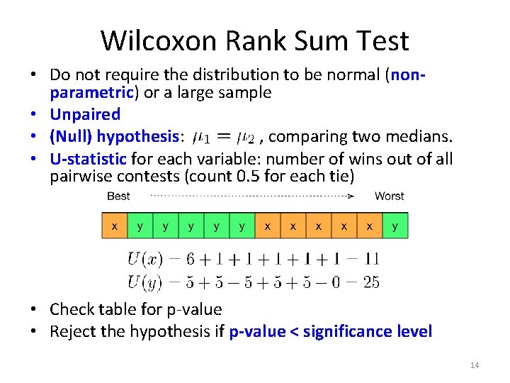
Wilcoxon Rank Sum Test • Do not require the distribution to be normal (nonparametric) or a large sample • Unpaired • (Null) hypothesis: , comparing two medians. • U-statistic for each variable: number of wins out of all pairwise contests (count 0. 5 for each tie) • Check table for p-value • Reject the hypothesis if p-value < significance level 14

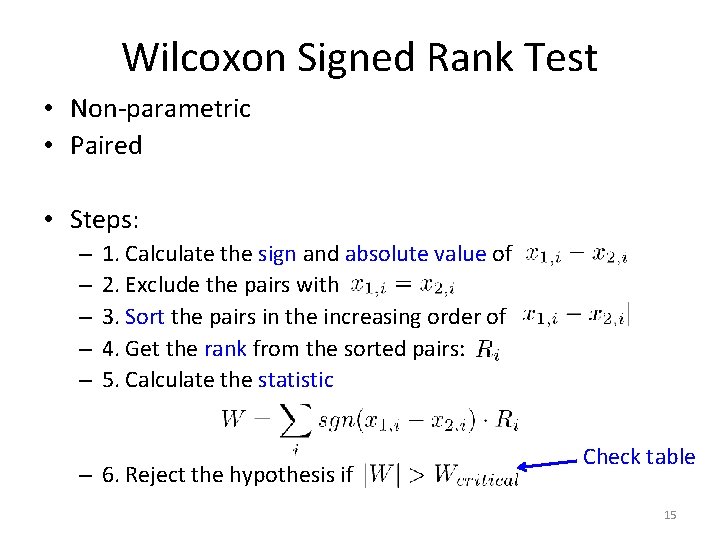
Wilcoxon Signed Rank Test • Non-parametric • Paired • Steps: – – – 1. Calculate the sign and absolute value of 2. Exclude the pairs with 3. Sort the pairs in the increasing order of 4. Get the rank from the sorted pairs: 5. Calculate the statistic – 6. Reject the hypothesis if Check table 15

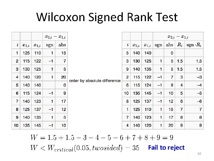
Wilcoxon Signed Rank Test Fail to reject 16

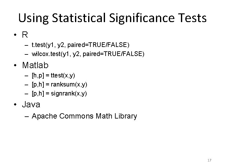
Using Statistical Significance Tests • R – t. test(y 1, y 2, paired=TRUE/FALSE) – wilcox. test(y 1, y 2, paired=TRUE/FALSE) • Matlab – [h, p] = ttest(x, y) – [p, h] = ranksum(x, y) – [p, h] = signrank(x, y) • Java – Apache Commons Math Library 17

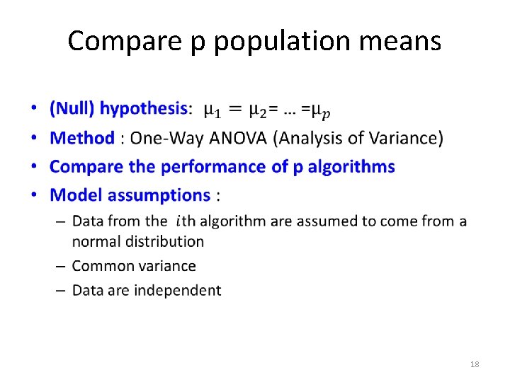
Compare p population means • 18

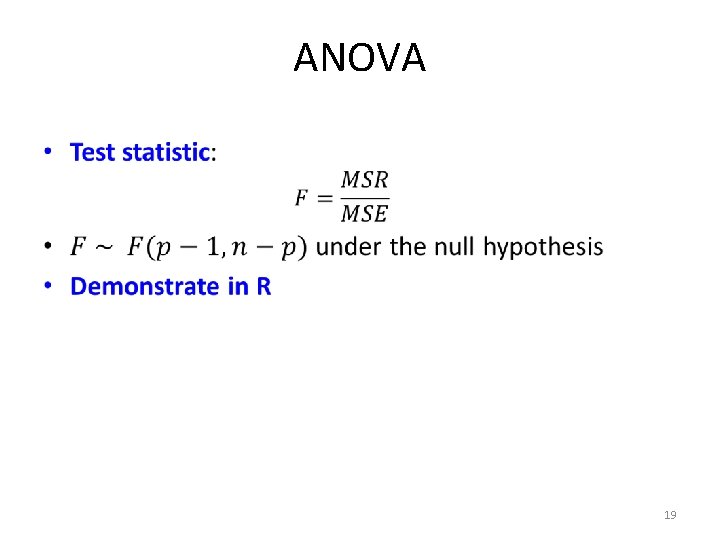
ANOVA • 19

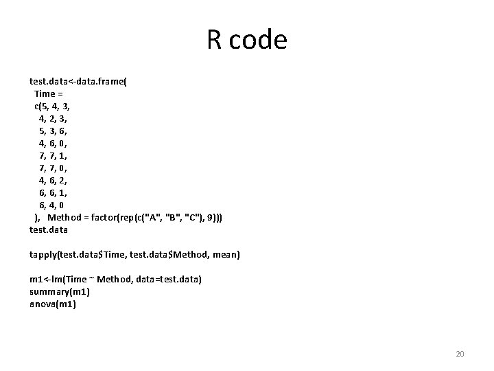
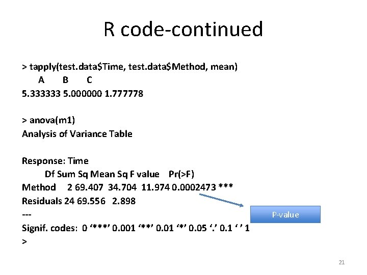
R code test. data<-data. frame( Time = c(5, 4, 3, 4, 2, 3, 5, 3, 6, 4, 6, 0, 7, 7, 1, 7, 7, 0, 4, 6, 2, 6, 6, 1, 6, 4, 0 ), Method = factor(rep(c("A", "B", "C"), 9))) test. data tapply(test. data$Time, test. data$Method, mean) m 1<-lm(Time ~ Method, data=test. data) summary(m 1) anova(m 1) 20

R code-continued > tapply(test. data$Time, test. data$Method, mean) A B C 5. 333333 5. 000000 1. 777778 > anova(m 1) Analysis of Variance Table Response: Time Df Sum Sq Mean Sq F value Pr(>F) Method 2 69. 407 34. 704 11. 974 0. 0002473 *** Residuals 24 69. 556 2. 898 --Signif. codes: 0 ‘***’ 0. 001 ‘**’ 0. 01 ‘*’ 0. 05 ‘. ’ 0. 1 ‘ ’ 1 > P-value 21

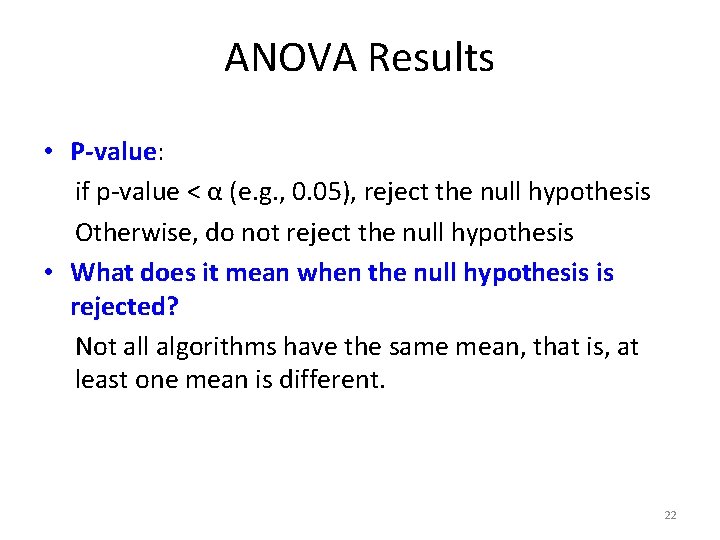
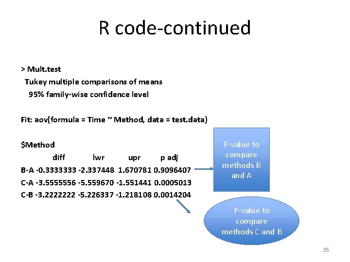
ANOVA Results • P-value: if p-value < α (e. g. , 0. 05), reject the null hypothesis Otherwise, do not reject the null hypothesis • What does it mean when the null hypothesis is rejected? Not all algorithms have the same mean, that is, at least one mean is different. 22

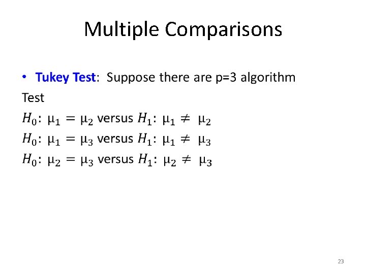
Multiple Comparisons • 23

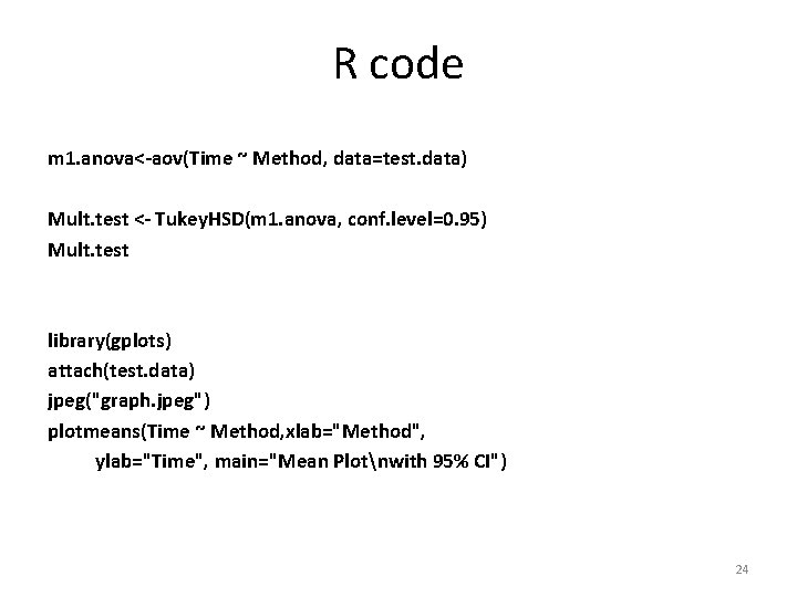
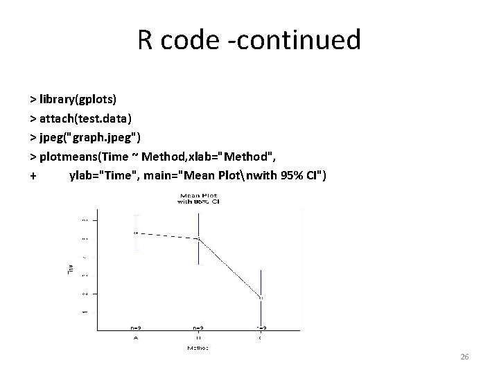
R code m 1. anova<-aov(Time ~ Method, data=test. data) Mult. test <- Tukey. HSD(m 1. anova, conf. level=0. 95) Mult. test library(gplots) attach(test. data) jpeg("graph. jpeg") plotmeans(Time ~ Method, xlab="Method", ylab="Time", main="Mean Plotnwith 95% CI") 24

R code-continued > Mult. test Tukey multiple comparisons of means 95% family-wise confidence level Fit: aov(formula = Time ~ Method, data = test. data) $Method diff lwr upr p adj B-A -0. 3333333 -2. 337448 1. 670781 0. 9096407 C-A -3. 5555556 -5. 559670 -1. 551441 0. 0005013 C-B -3. 2222222 -5. 226337 -1. 218108 0. 0014204 P-value to compare methods B and A P-value to compare methods C and B 25

R code -continued > library(gplots) > attach(test. data) > jpeg("graph. jpeg") > plotmeans(Time ~ Method, xlab="Method", + ylab="Time", main="Mean Plotnwith 95% CI") 26