Statistical programming in R Part 2 Point estimation

Statistical programming in R Part 2

Point estimation Topics covered Confidence interval Bootstrap

Point estimation

Point estimation One of the main goals of statistics is to estimate unknown parameters To approximate these parameters, we choose an estimator, which is simply any function of randomly sampled observations

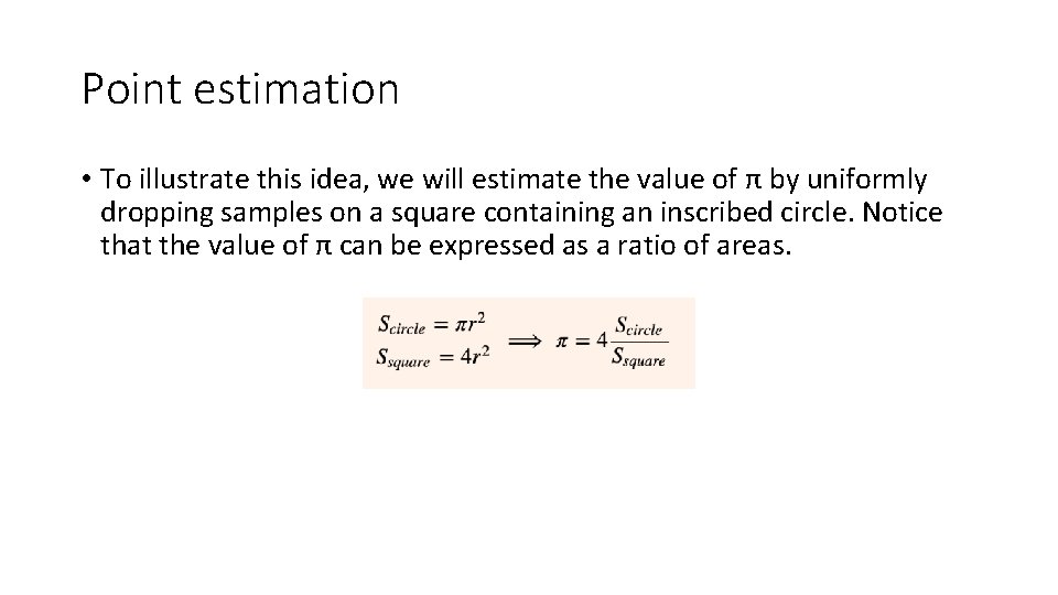
Point estimation • To illustrate this idea, we will estimate the value of π by uniformly dropping samples on a square containing an inscribed circle. Notice that the value of π can be expressed as a ratio of areas.

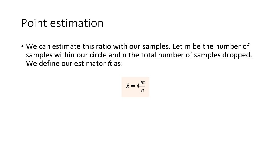
Point estimation • We can estimate this ratio with our samples. Let m be the number of samples within our circle and n the total number of samples dropped. We define our estimator π as:

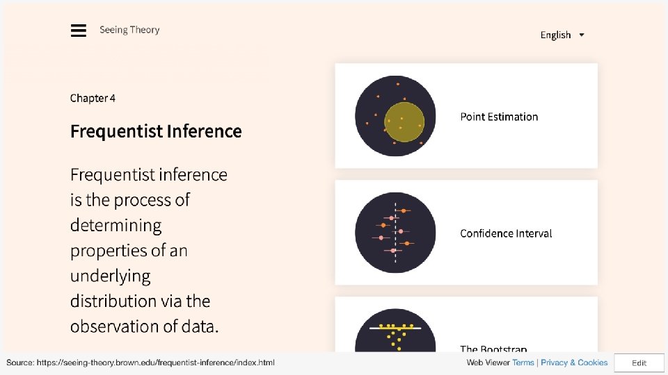
• https: //seeing-theory. brown. edu/basic-probability/index. html section 1

We may also sample from a reference population and see if our sample mean is a good approximation to the reference population In this case, we say that the sample mean is a point estimator of the true population parameter Point estimation in R Let us sample 10 samples from a normal distribution with mean of 0 and standard deviation of 1 sample <- rnorm(10, 0, 1) mean(sample) Is this sample mean close to the true population mean? Now, try with 100, 1000 and 10, 000 Are we getting closer?

Confidence interval

Another way of estimating parameter from a population is to define a range of possible values instead of just using 1 point estimate Confidence interval This range is an interval, and is associated with a confidence level The confidence level is the probability that this range will contain the true population parameter This is known formally as the confidence interval (CI)

• https: //seeing-theory. brown. edu/basic-probability/index. html section 1

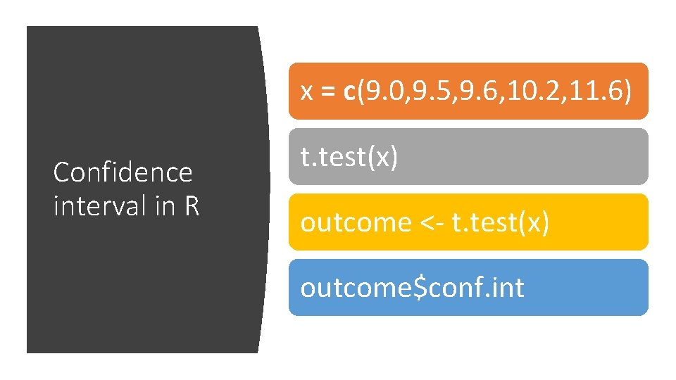
Confidence interval in R We will make some assumptions for what we might find in an experiment and find the resulting confidence interval using a normal distribution. In this example we will use a 95% confidence level and wish to find the confidence interval.

x = c(9. 0, 9. 5, 9. 6, 10. 2, 11. 6) Confidence interval in R t. test(x) outcome <- t. test(x) outcome$conf. int

Bootstrap

The computational technique known as the Bootstrap provides a convenient way to estimate properties of an estimator via resampling. Bootstrap In this example, we resample with replacement from the empirical distribution function in order to estimate the standard error of the sample mean.

• https: //seeing-theory. brown. edu/basic-probability/index. html section 1

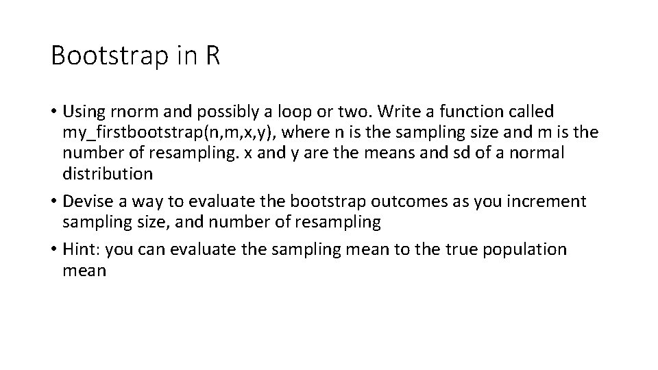
Bootstrap in R • Using rnorm and possibly a loop or two. Write a function called my_firstbootstrap(n, m, x, y), where n is the sampling size and m is the number of resampling. x and y are the means and sd of a normal distribution • Devise a way to evaluate the bootstrap outcomes as you increment sampling size, and number of resampling • Hint: you can evaluate the sampling mean to the true population mean

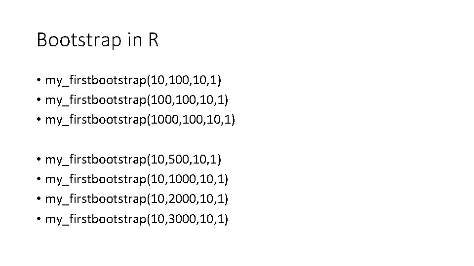
Bootstrap in R • my_firstbootstrap(10, 100, 10, 1) • my_firstbootstrap(1000, 10, 1) • my_firstbootstrap(10, 500, 1) • my_firstbootstrap(10, 1000, 1) • my_firstbootstrap(10, 2000, 1) • my_firstbootstrap(10, 3000, 1)

End of Segment Let’s take a break