Statistical Parametric Mapping SPM Talk I Spatial Preprocessing

General Linear Model (GLM) & Random Field Theory (RFT) Rik Henson With thanks to:

Overview f. MRI time-series kernel Design matrix Motion correction Smoothing General Linear Model Spatial

Some Terminology • SPM (“Statistical Parametric Mapping”) is a massively univariate approach - meaning

Some Terminology • SPM usually focused on “functional specialisation” - i. e. localising different

Overview 1. General Linear Model Design Matrix Estimation/Contrasts Covariates (eg global) Estimability/Correlation 2. f.

General Linear Model… • Parametric statistics • • • one sample t-test two sample

General Linear Model • Equation for single (and all) voxels: yj = xj 1

Matrix Formulation Equation for scan j Simultaneous equations for scans 1. . J Scans

General Linear Model (Estimation) • Estimate parameters from least squares fit to data, y:

GLM Estimation – Geometric Perspective y 1 x 1 1 y 2 = x

General Linear Model (Inference) • Specify contrast (hypothesis), c, a linear combination ^ of

Simple “ANOVA-like” Example rank(X)=3 • 12 scans, 3 conditions (1 -way ANOVA) yj =

Global Effects • May be variation in overall image intensity from scan to scan

Simple ANCOVA Example 1 2 4 5 rank(X)=4 • 12 scans, 3 conditions, 1

Global Effects (f. MRI) • • • Two types of scaling: Grand Mean scaling

A word on correlation/estimability • If any column of X is a linear combination

A word on correlation/estimability • When there is high (but not perfect) correlation between

A word on orthogonalisation • To remove correlation between two regressors, you can explicitly

A word on orthogonalisation X 1 X 2 b 1 = 0. 9 b

f. MRI Analysis 1. Scans are treated as a timeseries… …and can be filtered

(Epoch) f. MRI example… = b 1 + b 2 + (t) (box-car unconvolved)

Low frequency noise • Several causes of noise: aliasing – Physical (scanner drifts) –

(Epoch) f. MRI example… …fitted and adjusted data Raw f. MRI timeseries Adjusted data

Convolution with HRF Unconvolved fit Residuals Boxcar function Convolved fit = hæmodynamic response convolved

Temporal autocorrelation… • Because the data are typically correlated from one scan to the

Temporal autocorrelation (History) KY = KXb + K K ~ N(0, 2 V) V

Nonsphericity and Re. ML Scans • Nonsphericity means (kind of) that: C = cov(

Nonsphericity and Re. ML • Joint estimation of parameters and hyperparameters requires Re. ML

Nonsphericity and Re. ML 1. Voxels to be pooled collected by first-pass through data

T-contrasts and F-contrasts A T-contrast is a directional test of a unidimensional quantity (c

F-contrasts can test more… An F-contrast [1 0; 0 1] tests the sum of

B F: [1 -1] A A B T: [1 -1] B T/F-test decision spaces

T-contrasts A T statistic is ratio of a contrast, c. Tb, relative to the

F-contrasts An F statistic is a ratio of variances, e. g: the additional variance

F-contrasts Eg: do the movement parameters explain significant variability ? X 0 X 1

Multiple comparisons… • If n=100, 000 voxels tested with pu=0. 05 of falsely rejecting

Random Field Theory (RFT) • Consider SPM as lattice representation of continuous random field

Family. Wise Error • Want a “Family-wise Error” (FWE) Rate of, eg, 0. 05:

And so much more! Levels of Inference • Three levels of inference: – extreme

Small-volume correction (SVC) • If have an a priori region of interest, no need

Caveats for Random Field Theory Lattice Image Data • Always need sufficient smoothness: –FWHM

False Discovery Rate (FDR) • FWE (for height threshold) is probability of one or

Example Control of Per Comparison Rate at 10% 11. 3% 12. 5% 10. 8%

False Discovery Rate (FDR) • For any threshold, all voxels can be cross-classified: •

• • • Select desired limit q on FDR Order p-values, p(1) p(2)

Summary for False Disovery Rate • Adaptive, ie threshold depends on amount of signal:

Classical vs Bayesian Inference • In classic inference, the p-value represents the probability of

Parametric Empirical Bayes • Bayes rule: p( |y) = p(y| ) p( Posterior Likelihood

Hierarchical Models • In a hierarchical model, parameters of one level can be made

Posterior Probability Maps (PPMs) • Bayes rule: p( |y) = p(y| ) p( Posterior

PPMs vs SPMs • Activations greater than certain amount Voxels with non-zero activations •

Fixed vs. Random Effects • Subjects can be Fixed or Random variables • If

Two-stage “Summary Statistic” approach 2 nd-level (between-subject) 1 st-level (within-subject) b^2 ( ^ 2)

Limitations of 2 -stage approach • Summary statistic approach is a special case, valid

Slides: 78

Download presentation

Statistical Parametric Mapping (SPM) Talk I: Spatial Pre-processing & Morphometry Talk II: General Linear Model Talk III: Experimental Design & Efficiency Talk IV: EEG/MEG

General Linear Model (GLM) & Random Field Theory (RFT) Rik Henson With thanks to: Karl Friston, Andrew Holmes, Tom Nichols, Stefan Kiebel

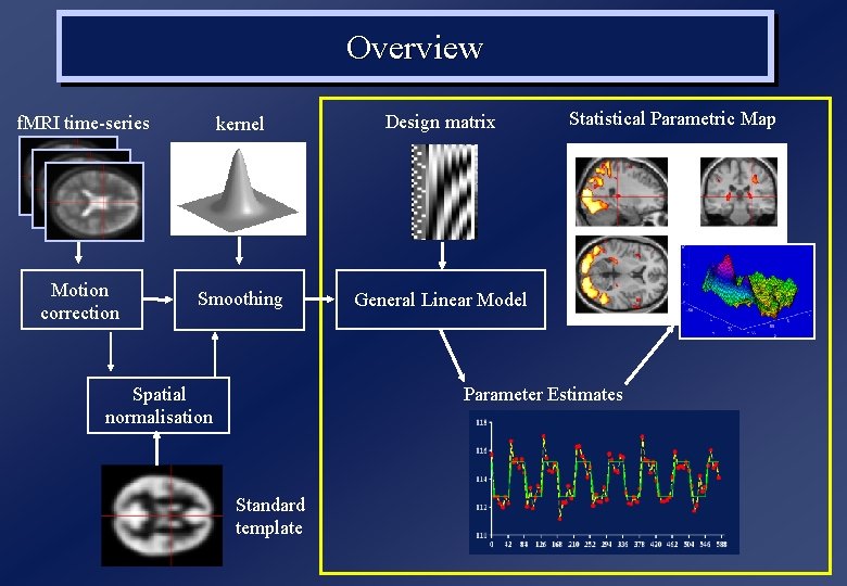
Overview f. MRI time-series kernel Design matrix Motion correction Smoothing General Linear Model Spatial normalisation Statistical Parametric Map Parameter Estimates Standard template

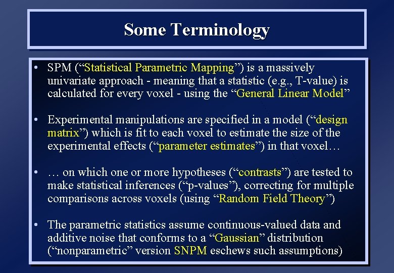
Some Terminology • SPM (“Statistical Parametric Mapping”) is a massively univariate approach - meaning that a statistic (e. g. , T-value) is calculated for every voxel - using the “General Linear Model” • Experimental manipulations are specified in a model (“design matrix”) which is fit to each voxel to estimate the size of the experimental effects (“parameter estimates”) in that voxel… • … on which one or more hypotheses (“contrasts”) are tested to make statistical inferences (“p-values”), correcting for multiple comparisons across voxels (using “Random Field Theory”) • The parametric statistics assume continuous-valued data and additive noise that conforms to a “Gaussian” distribution (“nonparametric” version SNPM eschews such assumptions)

Some Terminology • SPM usually focused on “functional specialisation” - i. e. localising different functions to different regions in the brain • One might also be interested in “functional integration” - how different regions (voxels) interact • Multivariate approaches work on whole images and can identify spatial/temporal patterns over voxels, without necessarily specifying a design matrix (PCA, ICA). . . • … or with an experimental design matrix (PLS, CVA), or with an explicit anatomical model of connectivity between regions “effective connectivity” - eg using Dynamic Causal Modelling

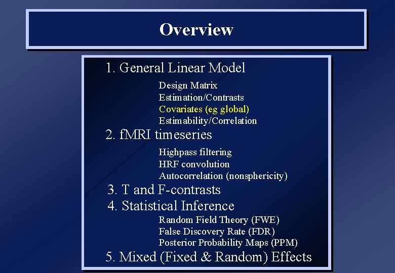
Overview 1. General Linear Model Design Matrix Estimation/Contrasts Covariates (eg global) Estimability/Correlation 2. f. MRI timeseries Highpass filtering HRF convolution Autocorrelation (nonsphericity) 3. T and F-contrasts 4. Statistical Inference Random Field Theory (FWE) False Discovery Rate (FDR) Posterior Probability Maps (PPM) 5. Mixed (Fixed & Random) Effects

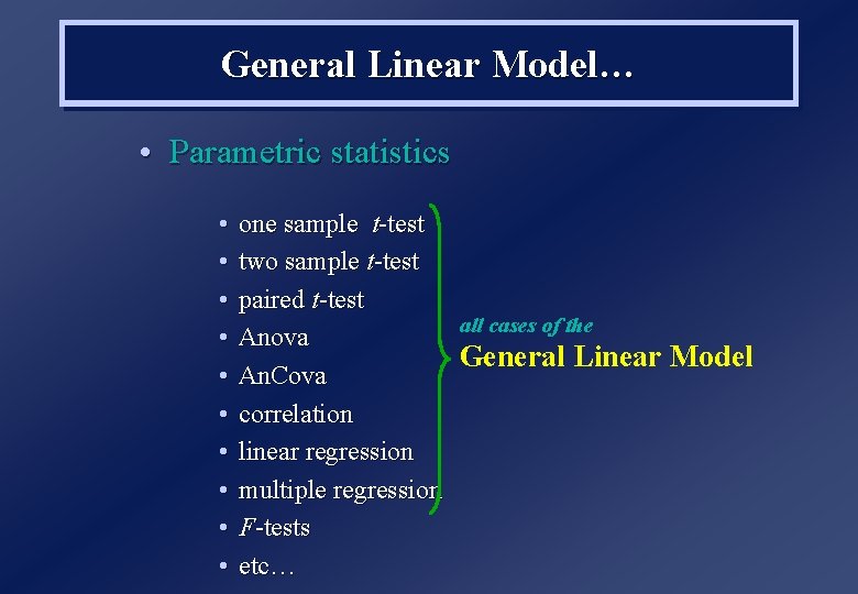
General Linear Model… • Parametric statistics • • • one sample t-test two sample t-test paired t-test all cases of the Anova General Linear Model An. Cova correlation linear regression multiple regression F-tests etc…

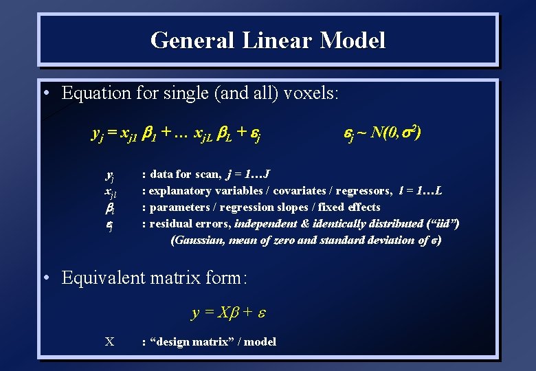
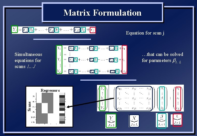
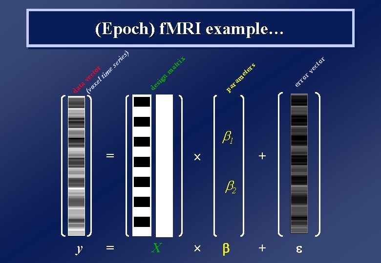
General Linear Model • Equation for single (and all) voxels: yj = xj 1 b 1 + … xj. L b. L + j yj xjl bl j : data for scan, j = 1…J : explanatory variables / covariates / regressors, l = 1…L : parameters / regression slopes / fixed effects : residual errors, independent & identically distributed (“iid”) (Gaussian, mean of zero and standard deviation of σ) • Equivalent matrix form: y = Xb + X j ~ N(0, s 2) : “design matrix” / model

Matrix Formulation Equation for scan j Simultaneous equations for scans 1. . J Scans Regressors …that can be solved for parameters b 1. . L

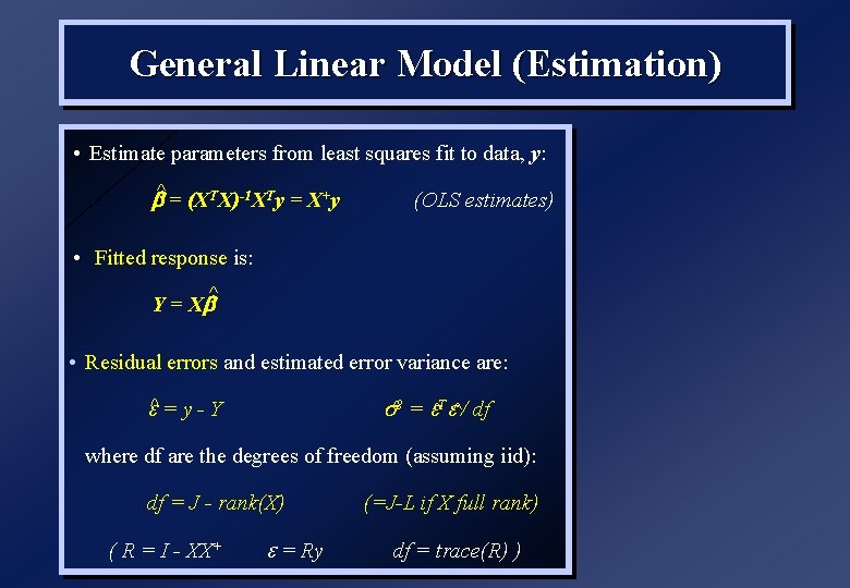
General Linear Model (Estimation) • Estimate parameters from least squares fit to data, y: b^ = (XTX)-1 XTy = X+y (OLS estimates) • Fitted response is: ^ Y = Xb • Residual errors and estimated error variance are: ^ = y - Y ^2 = ^T ^/ df where df are the degrees of freedom (assuming iid): df = J - rank(X) ( R = I - XX+ = Ry (=J-L if X full rank) df = trace(R) )

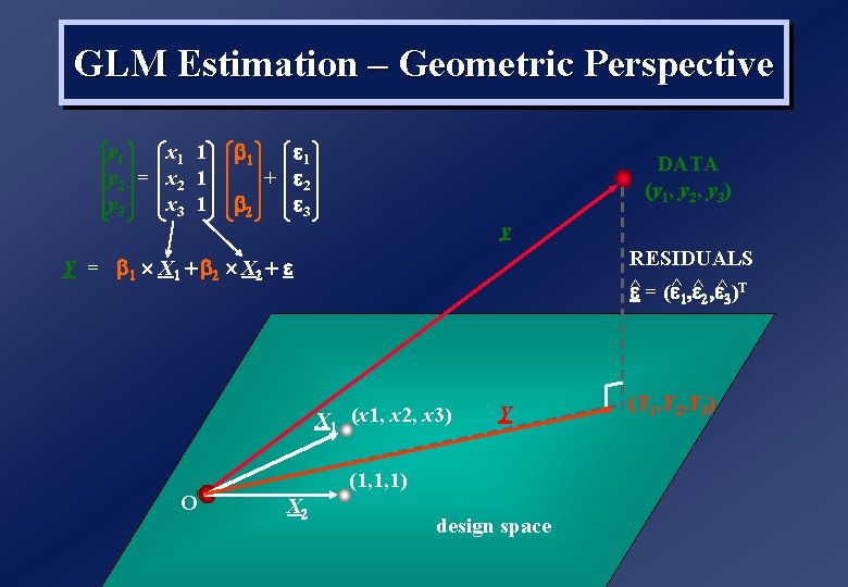
GLM Estimation – Geometric Perspective y 1 x 1 1 y 2 = x 2 1 y 3 x 3 1 1 1 + 2 2 3 DATA (y 1, y 2, y 3) y RESIDUALS ^ = ( ^1, ^2, ^3)T Y = 1 X 1 + 2 X 2 + X 1 (x 1, x 2, x 3) O Y (1, 1, 1) X 2 design space (Y 1, Y 2, Y 3)

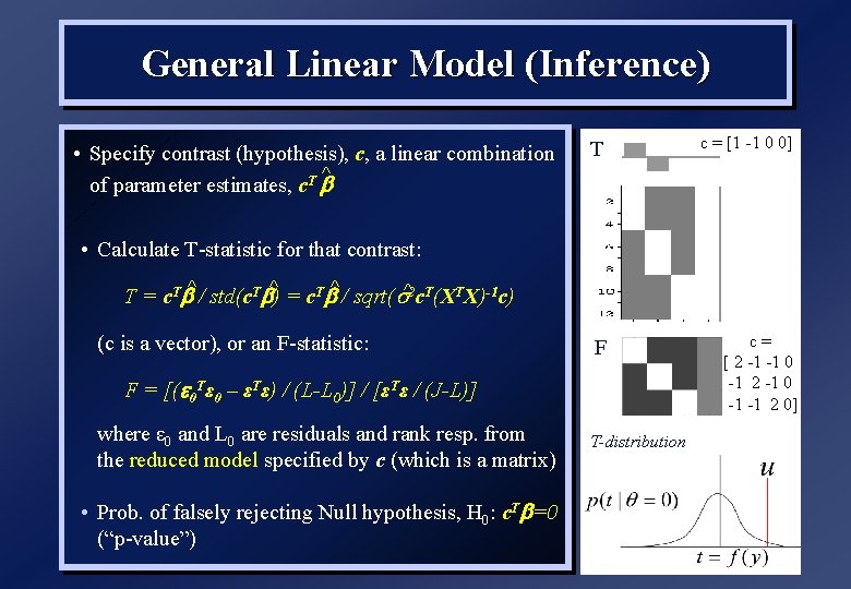
General Linear Model (Inference) • Specify contrast (hypothesis), c, a linear combination ^ of parameter estimates, c. T b T c = [1 -1 0 0] • Calculate T-statistic for that contrast: ^ ^ T = c. Tb^ / std(c. Tb) = c. Tb / sqrt( ^2 c. T(XTX)-1 c) (c is a vector), or an F-statistic: F F = [( 0 Tε 0 – εTε) / (L-L 0)] / [εTε / (J-L)] where ε 0 and L 0 are residuals and rank resp. from the reduced model specified by c (which is a matrix) • Prob. of falsely rejecting Null hypothesis, H 0: c. Tb=0 (“p-value”) T-distribution c= [ 2 -1 -1 0 -1 2 -1 0 -1 -1 2 0]

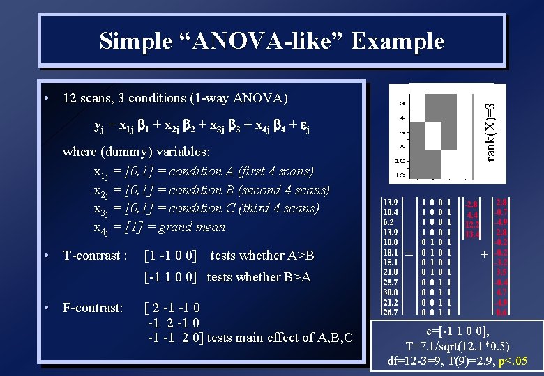
Simple “ANOVA-like” Example rank(X)=3 • 12 scans, 3 conditions (1 -way ANOVA) yj = x 1 j 1 + x 2 j 2 + x 3 j 3 + x 4 j 4 + j where (dummy) variables: x 1 j = [0, 1] = condition A (first 4 scans) x 2 j = [0, 1] = condition B (second 4 scans) x 3 j = [0, 1] = condition C (third 4 scans) x 4 j = [1] = grand mean • T-contrast : [1 -1 0 0] tests whether A>B [-1 1 0 0] tests whether B>A • F-contrast: [ 2 -1 -1 0 -1 2 -1 0 -1 -1 2 0] tests main effect of A, B, C 13. 9 10. 4 6. 2 13. 9 18. 0 18. 1 15. 1 21. 8 25. 7 30. 8 21. 2 26. 7 = 1 1 1 1 0 0 0 0 0 0 1 1 1 1 -2. 8 4. 4 12. 2 13. 4 + 2. 8 -0. 7 -4. 9 2. 8 -0. 2 -3. 2 3. 5 -0. 4 4. 7 -4. 9 0. 6 c=[-1 1 0 0], T=7. 1/sqrt(12. 1*0. 5) df=12 -3=9, T(9)=2. 9, p<. 05

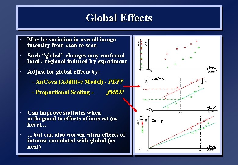
Global Effects • May be variation in overall image intensity from scan to scan • Such “global” changes may confound local / regional induced by experiment global • Adjust for global effects by: - An. Cova (Additive Model) - PET? - Proportional Scaling - An. Cova f. MRI? • Can improve statistics when orthogonal to effects of interest (as here)… • …but can also worsen when effects of interest correlated with global (as next) global Scaling global

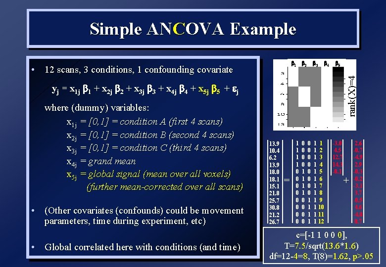
Simple ANCOVA Example 1 2 4 5 rank(X)=4 • 12 scans, 3 conditions, 1 confounding covariate 3 yj = x 1 j 1 + x 2 j 2 + x 3 j 3 + x 4 j 4 + x 5 j 5 + j where (dummy) variables: x 1 j = [0, 1] = condition A (first 4 scans) x 2 j = [0, 1] = condition B (second 4 scans) x 3 j = [0, 1] = condition C (third 4 scans) x 4 j = grand mean x 5 j = global signal (mean over all voxels) (further mean-corrected over all scans) • (Other covariates (confounds) could be movement parameters, time during experiment, etc) • Global correlated here with conditions (and time) 13. 9 10. 4 6. 2 13. 9 18. 0 18. 1 15. 1 21. 8 25. 7 30. 8 21. 2 26. 7 = 1 1 1 1 0 0 0 0 0 0 1 1 1 1 2 1 3 1 4 1 5 1 6 1 7 1 8 1 9 1 10 1 11 1 12 -3. 0 4. 5 12. 7 14. 3 -0. 1 + 2. 6 -0. 7 -4. 9 2. 9 -0. 3 -0. 2 -3. 1 3. 7 -0. 5 4. 6 -4. 8 0. 7 c=[-1 1 0 0 0], T=7. 5/sqrt(13. 6*1. 6) df=12 -4=8, T(8)=1. 62, p>. 05

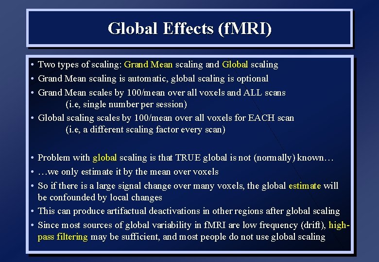
Global Effects (f. MRI) • • • Two types of scaling: Grand Mean scaling and Global scaling Grand Mean scaling is automatic, global scaling is optional Grand Mean scales by 100/mean over all voxels and ALL scans (i. e, single number per session) • Global scaling scales by 100/mean over all voxels for EACH scan (i. e, a different scaling factor every scan) • • • Problem with global scaling is that TRUE global is not (normally) known… …we only estimate it by the mean over voxels So if there is a large signal change over many voxels, the global estimate will be confounded by local changes • This can produce artifactual deactivations in other regions after global scaling • Since most sources of global variability in f. MRI are low frequency (drift), highpass filtering may be sufficient, and most people do not use global scaling

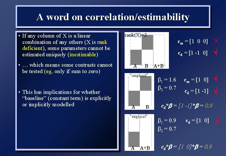
A word on correlation/estimability • If any column of X is a linear combination of any others (X is rank deficient), some parameters cannot be estimated uniquely (inestimable) rank(X)=2 • … which means some contrasts cannot be tested (eg, only if sum to zero) A • This has implications for whether “baseline” (constant term) is explicitly or implicitly modelled B “implicit” A B “explicit” A A+B cm = [1 0 0] cd = [1 -1 0] cm = [1 0] cd = [1 -1] A+B b 1 = 1. 6 b 2 = 0. 7 cd*b = [1 -1]*b = 0. 9 b 1 = 0. 9 b 2 = 0. 7 cd = [1 0] cd*b = [1 0]*b = 0. 9

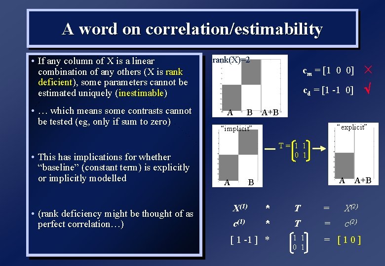
A word on correlation/estimability • If any column of X is a linear combination of any others (X is rank deficient), some parameters cannot be estimated uniquely (inestimable) rank(X)=2 • … which means some contrasts cannot be tested (eg, only if sum to zero) A • This has implications for whether “baseline” (constant term) is explicitly or implicitly modelled • (rank deficiency might be thought of as perfect correlation…) B cm = [1 0 0] cd = [1 -1 0] A+B “explicit” “implicit” T= 1 1 0 1 A A B A+B X(1) * T = X(2) c(1) * T = c(2) 1 1 0 1 = [10] [ 1 -1 ] *

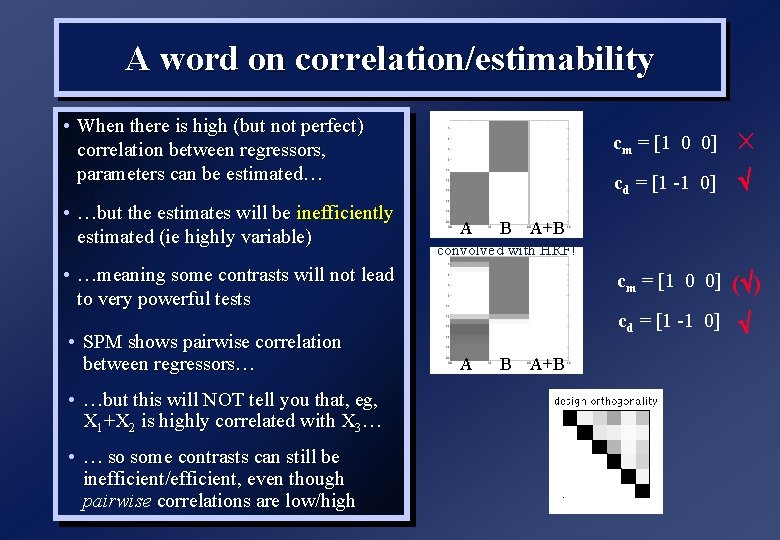
A word on correlation/estimability • When there is high (but not perfect) correlation between regressors, parameters can be estimated… • …but the estimates will be inefficiently estimated (ie highly variable) A B • …but this will NOT tell you that, eg, X 1+X 2 is highly correlated with X 3… • … so some contrasts can still be inefficient/efficient, even though pairwise correlations are low/high cd = [1 -1 0] cm = [1 0 0] ( ) cd = [1 -1 0] A+B convolved with HRF! • …meaning some contrasts will not lead to very powerful tests • SPM shows pairwise correlation between regressors… cm = [1 0 0] A B A+B

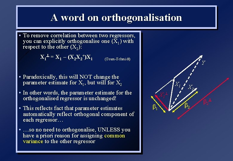
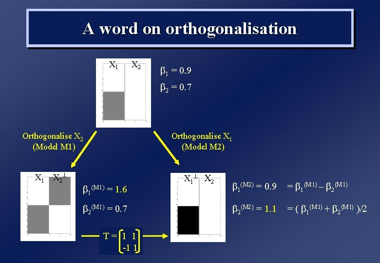
A word on orthogonalisation • To remove correlation between two regressors, you can explicitly orthogonalise one (X 1) with respect to the other (X 2): X 1^ = X 1 – (X 2 X 2+)X 1 (Gram-Schmidt) Y • Paradoxically, this will NOT change the parameter estimate for X 1, but will for X 2 X 1 • In other words, the parameter estimate for the orthogonalised regressor is unchanged! • This reflects fact that parameter estimates automatically reflect orthogonal component of each regressor… • …so no need to orthogonalise, UNLESS you have a priori reason for assigning common variance to the other regressor X 1 ^ b 1 X 2 b 2 ^

A word on orthogonalisation X 1 X 2 b 1 = 0. 9 b 2 = 0. 7 Orthogonalise X 2 (Model M 1) X 1 X 2 ^ Orthogonalise X 1 (Model M 2) b 1(M 1) = 1. 6 b 2(M 1) = 0. 7 T= 1 1 -1 1 X 1 ^ X 2 b 1(M 2) = 0. 9 = b 1(M 1 – b 2(M 1 b 2(M = 1. 1 = ( b 1(M 1 + b 2(M 1 /

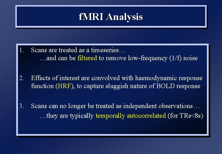
f. MRI Analysis 1. Scans are treated as a timeseries… …and can be filtered to remove low-frequency (1/f) noise 2. Effects of interest are convolved with haemodynamic response function (HRF), to capture sluggish nature of BOLD response 3. Scans can no longer be treated as independent observations… …they are typically temporally autocorrelated (for TRs<8 s)

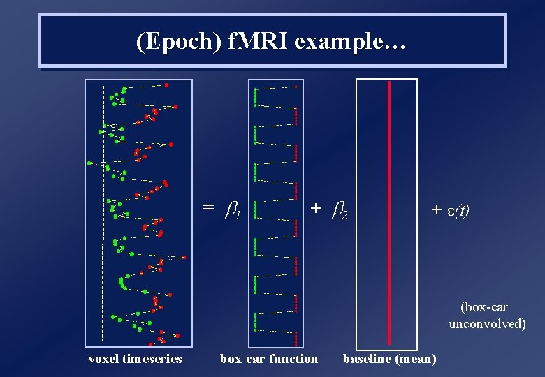
(Epoch) f. MRI example… = b 1 + b 2 + (t) (box-car unconvolved) voxel timeseries box-car function baseline (mean)

y = = X r to ec rv ro er s x ri at er m et m ra pa n de sig s) ie er (v vec ox to el r tim es ta da (Epoch) f. MRI example… b 1 + b 2 +

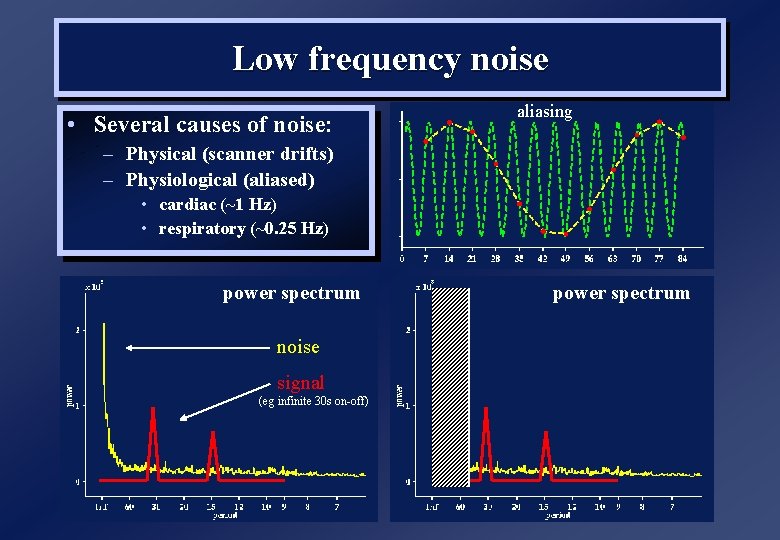
Low frequency noise • Several causes of noise: aliasing – Physical (scanner drifts) – Physiological (aliased) • cardiac (~1 Hz) • respiratory (~0. 25 Hz) power spectrum noise signal (eg infinite 30 s on-off) power spectrum highpass filter

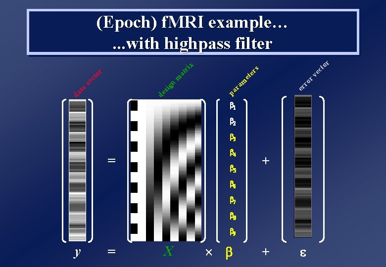
to ec s rv er et ro m er ra pa da ta de sig n ve m ct at or ri x r (Epoch) f. MRI example…. . . with highpass filter 1 2 3 4 = 5 + 6 7 8 9 y = X +

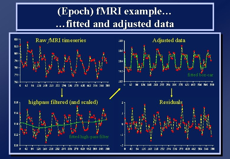
(Epoch) f. MRI example… …fitted and adjusted data Raw f. MRI timeseries Adjusted data fitted box-car highpass filtered (and scaled) fitted high-pass filter Residuals

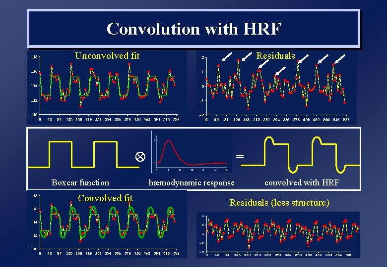
Convolution with HRF Unconvolved fit Residuals Boxcar function Convolved fit = hæmodynamic response convolved with HRF Residuals (less structure)

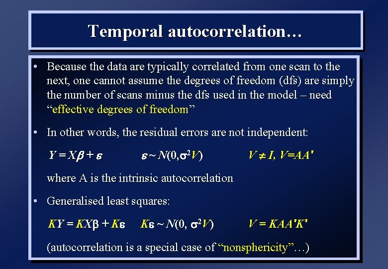
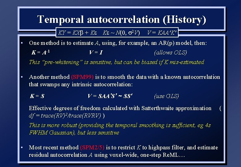
Temporal autocorrelation… • Because the data are typically correlated from one scan to the next, one cannot assume the degrees of freedom (dfs) are simply the number of scans minus the dfs used in the model – need “effective degrees of freedom” • In other words, the residual errors are not independent: Y = Xb + ~ N(0, s 2 V) V I, V=AA' where A is the intrinsic autocorrelation • Generalised least squares: KY = KX + K K ~ N(0, s 2 V) V = KAA'K' (autocorrelation is a special case of “nonsphericity”…)

Temporal autocorrelation (History) KY = KXb + K K ~ N(0, 2 V) V = KAA'K' • One method is to estimate A, using, for example, an AR(p) model, then: K = A-1 V=I (allows OLS) This “pre-whitening” is sensitive, but can be biased if K mis-estimated • Another method (SPM 99) is to smooth the data with a known autocorrelation that swamps any intrinsic autocorrelation: K=S V = SAA'S’ ~ SS‘ (use GLS) Effective degrees of freedom calculated with Satterthwaite approximation df = trace(RV)2/trace(RVRV) ) This is more robust (providing the temporal smoothing is sufficient, eg 4 s FWHM Gaussian), but less sensitive • Most recent method (SPM 2/5) is to restrict K to highpass filter, and estimate residual autocorrelation A using voxel-wide, one-step Re. ML… (

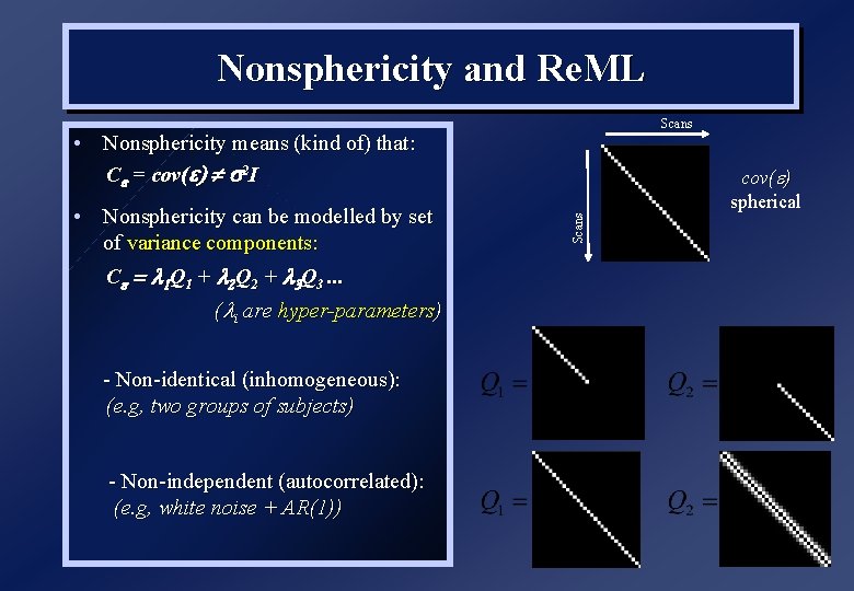
Nonsphericity and Re. ML Scans • Nonsphericity means (kind of) that: C = cov( ) s 2 I ( i are hyper-parameters) - Non-identical (inhomogeneous): (e. g, two groups of subjects) - Non-independent (autocorrelated): (e. g, white noise + AR(1)) Scans • Nonsphericity can be modelled by set of variance components: C = 1 Q 1 + 2 Q 2 + 3 Q 3. . . cov( ) spherical

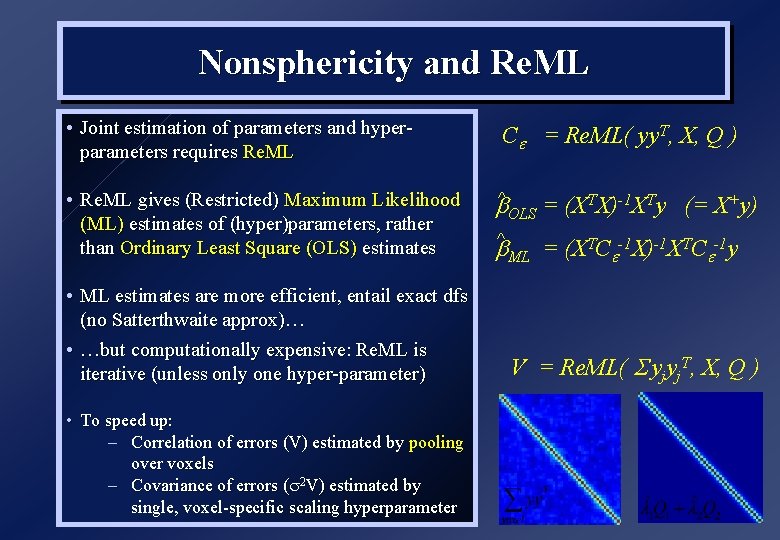
Nonsphericity and Re. ML • Joint estimation of parameters and hyperparameters requires Re. ML • Re. ML gives (Restricted) Maximum Likelihood (ML) estimates of (hyper)parameters, rather than Ordinary Least Square (OLS) estimates • ML estimates are more efficient, entail exact dfs (no Satterthwaite approx)… • …but computationally expensive: Re. ML is iterative (unless only one hyper-parameter) • To speed up: – Correlation of errors (V) estimated by pooling over voxels – Covariance of errors ( 2 V) estimated by single, voxel-specific scaling hyperparameter C = Re. ML( yy. T, X, Q ) b^ OLS = (XTX)-1 XTy (= X+y) b^ ML = (XTC -1 X)-1 XTC -1 y V = Re. ML( yjyj. T, X, Q )

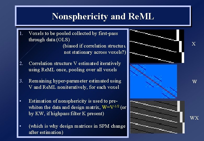
Nonsphericity and Re. ML 1. Voxels to be pooled collected by first-pass through data (OLS) B (biased if correlation structure not stationary across voxels? ) X 2. Correlation structure V estimated iteratively using Re. ML once, pooling over all voxels 3. Remaining hyper-parameter estimated using V and Re. ML noniteratively, for each voxel • • Estimation of nonsphericity is used to prewhiten the data and design matrix, W=V-1/2 (or by KW, if highpass filter K present) (which is why design matrices in SPM change after estimation) W WX

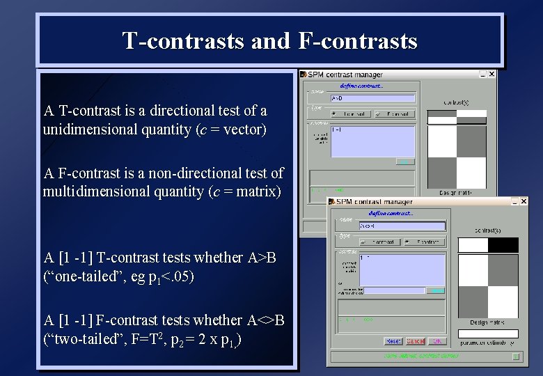
T-contrasts and F-contrasts A T-contrast is a directional test of a unidimensional quantity (c = vector) A F-contrast is a non-directional test of multidimensional quantity (c = matrix) A [1 -1] T-contrast tests whether A>B (“one-tailed”, eg p 1<. 05) A [1 -1] F-contrast tests whether A<>B (“two-tailed”, F=T 2, p 2 = 2 x p 1, )

F-contrasts can test more… An F-contrast [1 0; 0 1] tests the sum of squares of A and B (loosely the “union” of A and B; loosely “A and/or B”) An F-contrast [1 -1 0; 0 1 -1] tests “main effect” of a 3 -level factor in an ANOVA Some further notes on F-contrasts: 1. Sign irrelevant (for stats; affects plots) [1 0; 0 1] ≡ [-1 0; 0 -1] ≡ [1 0; 0 -1] 2. Scale/row order irrelevant (for stats) [1 0; 0 1] ≡ [2 0; 0 2] ≡ [0 1; 1 0] 3. Rank relevant (for stats; affects plots): [1 -1 0; 0 1 -1] ≡ [1 1 -2; 1 -1 0] ≡ [2 -1 -1; -1 2 -1; -1 -1 2] (latter is SPM’s “effects of interest”)

B F: [1 -1] A A B T: [1 -1] B T/F-test decision spaces F: [1 0 0 1] A

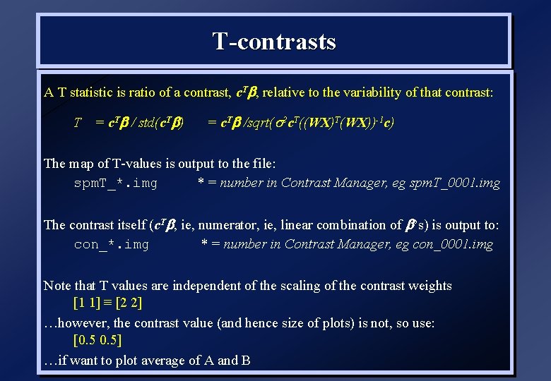
T-contrasts A T statistic is ratio of a contrast, c. Tb, relative to the variability of that contrast: T = c. Tb / std(c. Tb) = c. Tb /sqrt( 2 c. T((WX)T(WX))-1 c) The map of T-values is output to the file: spm. T_*. img * = number in Contrast Manager, eg spm. T_0001. img The contrast itself (c. Tb, ie, numerator, ie, linear combination of b’s) is output to: con_*. img * = number in Contrast Manager, eg con_0001. img Note that T values are independent of the scaling of the contrast weights [1 1] ≡ [2 2] …however, the contrast value (and hence size of plots) is not, so use: [0. 5] …if want to plot average of A and B

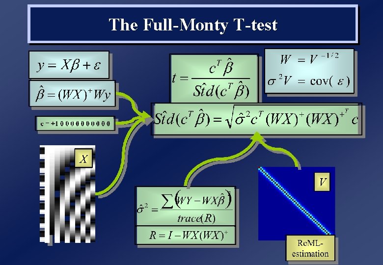
The Full-Monty T-test

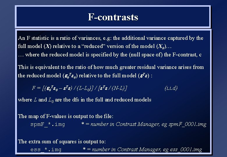
F-contrasts An F statistic is a ratio of variances, e. g: the additional variance captured by the full model (X) relative to a “reduced” version of the model (X 0)… … where the reduced model is specified by the (null space of) the F-contrast, c This is equivalent to the ratio of how much greater residual variance arises from the reduced model ( 0 Tε 0) relative to the full model ( Tε) : F = [( 0 Tε 0 – εTε) / (L-L 0)] / [εTε / (N-L)] (i. i. d) where L and L 0 are the dfs in the full and reduced models The map of F-values is output to the file: spm. F_*. img * = number in Contrast Manager, eg spm. F_0001. img The extra sum of squares is output to: ess_*. img * = number in Contrast Manager, eg ess_0001. img

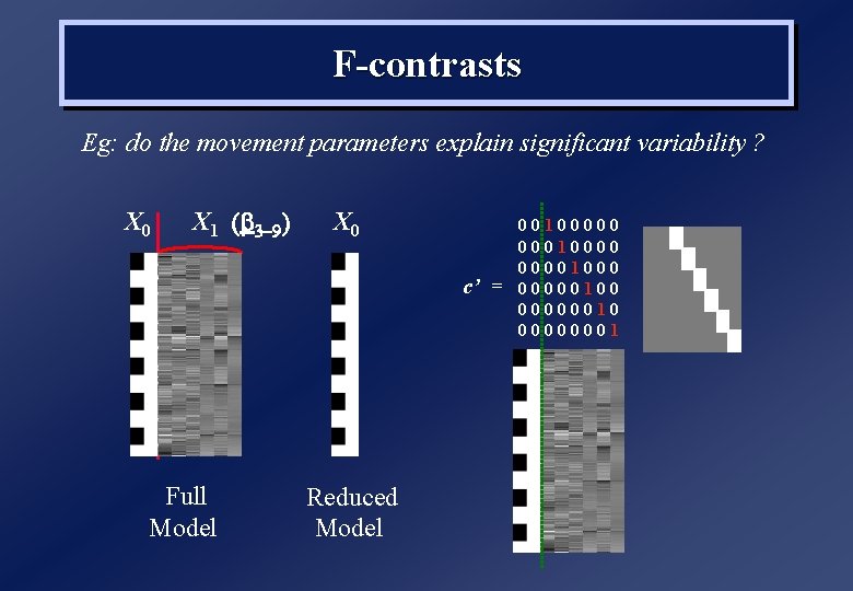
F-contrasts Eg: do the movement parameters explain significant variability ? X 0 X 1 ( 3 -9) X 0 c’ = Full Model Reduced Model 00100000 000100001000 00000100 00000010 00000001

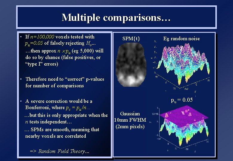
Multiple comparisons… • If n=100, 000 voxels tested with pu=0. 05 of falsely rejecting Ho. . . …then approx n pu (eg 5, 000) will do so by chance (false positives, or “type I” errors) SPM{t} Eg random noise • Therefore need to “correct” p-values for number of comparisons • A severe correction would be a Bonferroni, where pc = pu /n… …but this is only appropriate when the n tests independent… … SPMs are smooth, meaning that nearby voxels are correlated => Random Field Theory. . . pu = 0. 05 Gaussian 10 mm FWHM (2 mm pixels)

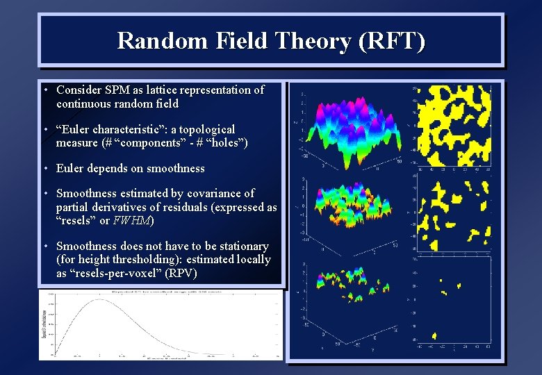
Random Field Theory (RFT) • Consider SPM as lattice representation of continuous random field • “Euler characteristic”: a topological measure (# “components” - # “holes”) • Euler depends on smoothness • Smoothness estimated by covariance of partial derivatives of residuals (expressed as “resels” or FWHM) • Smoothness does not have to be stationary (for height thresholding): estimated locally as “resels-per-voxel” (RPV)

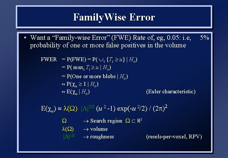
Family. Wise Error • Want a “Family-wise Error” (FWE) Rate of, eg, 0. 05: i. e, probability of one or more false positives in the volume FWER = P(FWE) = P( i {Ti u} | Ho) = P( maxi Ti u | Ho) = P(One or more blobs | Ho) P( u 1 | Ho) E( u | Ho) 5% (Euler characteristic) E( u) ( ) | |1/2 (u 2 -1) exp(-u 2/2) / (2 )2 ( | |1/2 Search region R 3 volume roughness (resels-per-voxel, RPV)

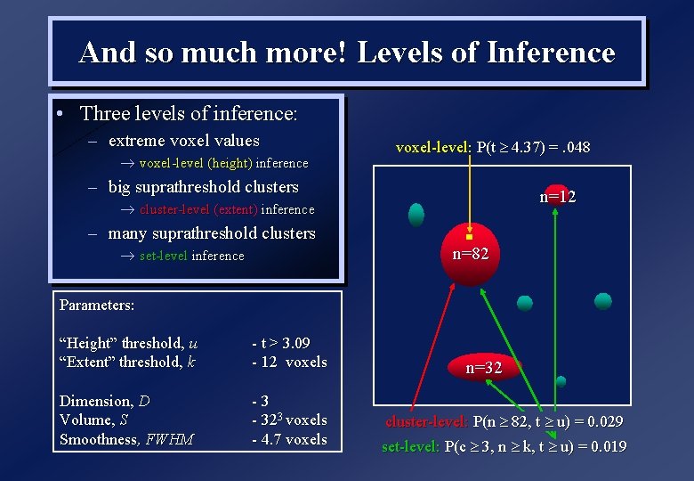
And so much more! Levels of Inference • Three levels of inference: – extreme voxel values voxel-level (height) inference voxel-level: P(t 4. 37) =. 048 – big suprathreshold clusters n=12 cluster-level (extent) inference – many suprathreshold clusters set-level inference n=82 Parameters: “Height” threshold, u “Extent” threshold, k - t > 3. 09 - 12 voxels Dimension, D Volume, S Smoothness, FWHM -3 - 323 voxels - 4. 7 voxels n=32 cluster-level: P(n 82, t u) = 0. 029 set-level: P(c 3, n k, t u) = 0. 019

Example SPM window

(Spatial) Specificity vs. Sensitivity

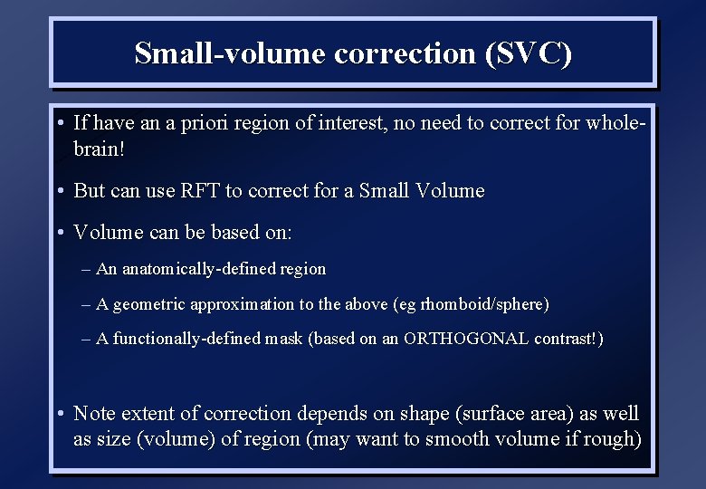
Small-volume correction (SVC) • If have an a priori region of interest, no need to correct for wholebrain! • But can use RFT to correct for a Small Volume • Volume can be based on: – An anatomically-defined region – A geometric approximation to the above (eg rhomboid/sphere) – A functionally-defined mask (based on an ORTHOGONAL contrast!) • Note extent of correction depends on shape (surface area) as well as size (volume) of region (may want to smooth volume if rough)

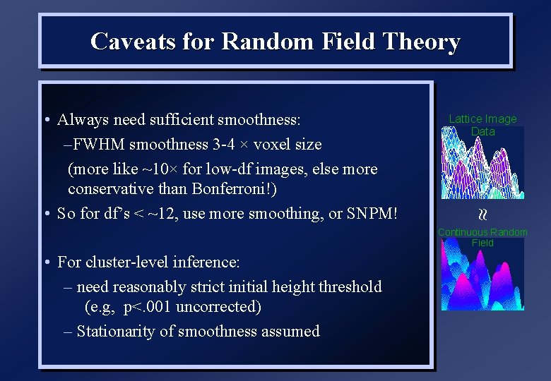
Caveats for Random Field Theory Lattice Image Data • Always need sufficient smoothness: –FWHM smoothness 3 -4 × voxel size (more like ~10× for low-df images, else more conservative than Bonferroni!) • So for df’s < ~12, use more smoothing, or SNPM! Continuous Random Field • For cluster-level inference: – need reasonably strict initial height threshold (e. g, p<. 001 uncorrected) – Stationarity of smoothness assumed

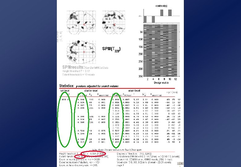
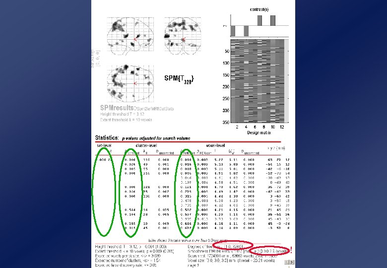
Example SPM window !

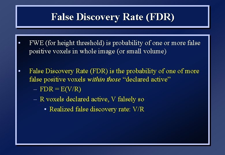
False Discovery Rate (FDR) • FWE (for height threshold) is probability of one or more false positive voxels in whole image (or small volume) • False Discovery Rate (FDR) is the probability of one of more false positive voxels within those “declared active” – FDR = E(V/R) – R voxels declared active, V falsely so • Realized false discovery rate: V/R

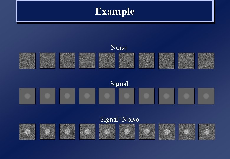
Example Noise Signal+Noise

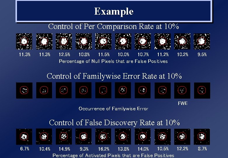
Example Control of Per Comparison Rate at 10% 11. 3% 12. 5% 10. 8% 11. 5% 10. 0% 10. 7% 11. 2% Percentage of Null Pixels that are False Positives 10. 2% 9. 5% Control of Familywise Error Rate at 10% FWE Occurrence of Familywise Error Control of False Discovery Rate at 10% 6. 7% 10. 4% 10. 5% 12. 2% 14. 9% 9. 3% 16. 2% 13. 8% 14. 0% Percentage of Activated Pixels that are False Positives 8. 7%

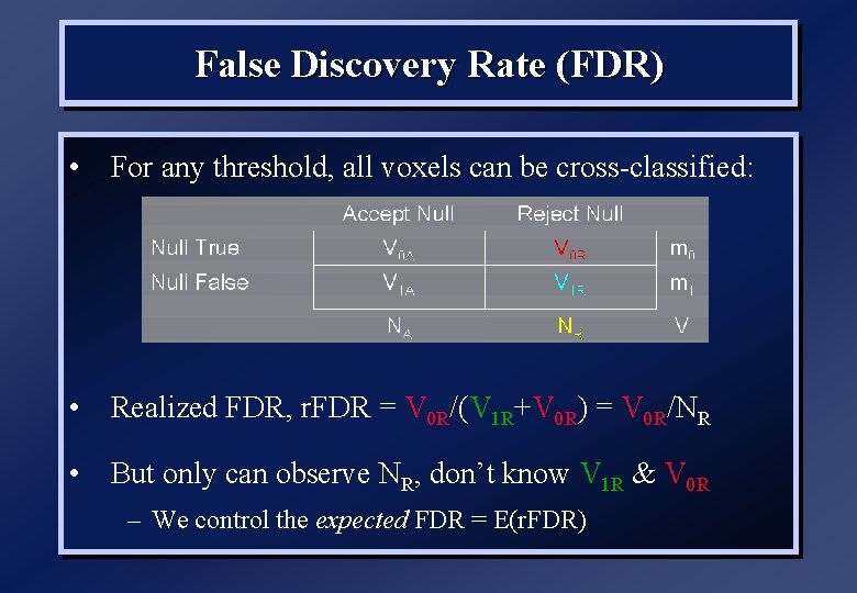
False Discovery Rate (FDR) • For any threshold, all voxels can be cross-classified: • Realized FDR, r. FDR = V 0 R/(V 1 R+V 0 R) = V 0 R/NR • But only can observe NR, don’t know V 1 R & V 0 R – We control the expected FDR = E(r. FDR)

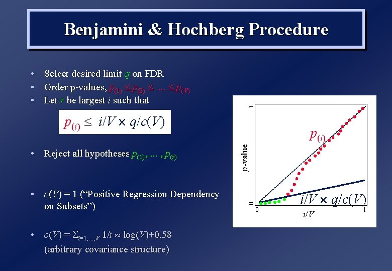
• • • Select desired limit q on FDR Order p-values, p(1) p(2) . . . p(V) Let r be largest i such that 1 Benjamini & Hochberg Procedure p(i) i/V q/c(V) • c(V) = 1 (“Positive Regression Dependency on Subsets”) • c(V) = i=1, . . . , V 1/i log(V)+0. 58 (arbitrary covariance structure) p-value i/V q/c(V) 0 • Reject all hypotheses p(1), . . . , p(r) p(i) 0 i/V 1

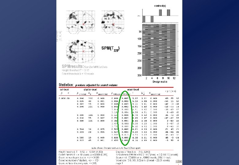
Example SPM window

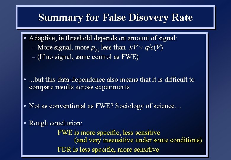
Summary for False Disovery Rate • Adaptive, ie threshold depends on amount of signal: – More signal, more p(i) less than i/V q/c(V) – (If no signal, same control as FWE) • . . . but this data-dependence also means that it is difficult to compare results across experiments • Not as conventional as FWE? Sociology of science… • Rough conclusion: FWE is more specific, less sensitive (and very insensitive under some conditions) FDR is less specific, more sensitive

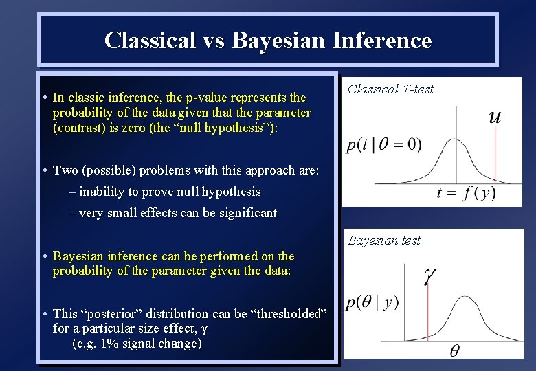
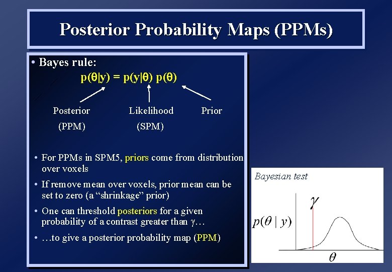
Classical vs Bayesian Inference • In classic inference, the p-value represents the probability of the data given that the parameter (contrast) is zero (the “null hypothesis”): Classical T-test • Two (possible) problems with this approach are: – inability to prove null hypothesis – very small effects can be significant • Bayesian inference can be performed on the probability of the parameter given the data: • This “posterior” distribution can be “thresholded” for a particular size effect, γ (e. g. 1% signal change) Bayesian test

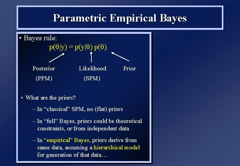
Parametric Empirical Bayes • Bayes rule: p( |y) = p(y| ) p( Posterior Likelihood (PPM) (SPM) Prior • What are the priors? – In “classical” SPM, no (flat) priors – In “full” Bayes, priors could be theoretical constraints, or from independent data – In “empirical” Bayes, priors derive from same data, assuming a hierarchical model for generation of that data…

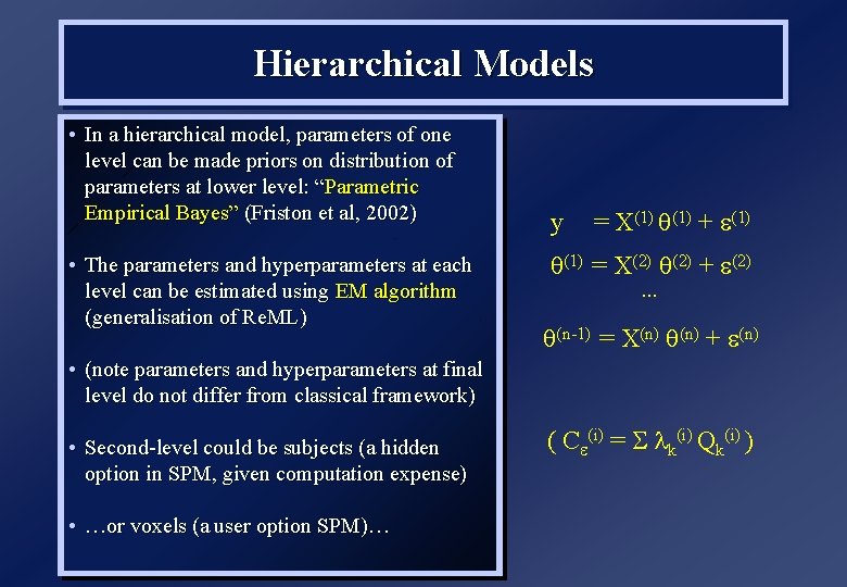
Hierarchical Models • In a hierarchical model, parameters of one level can be made priors on distribution of parameters at lower level: “Parametric Empirical Bayes” (Friston et al, 2002) • The parameters and hyperparameters at each level can be estimated using EM algorithm (generalisation of Re. ML) y = X(1) + (1) = X(2) + (2) … (n-1) = X(n) + (n) • (note parameters and hyperparameters at final level do not differ from classical framework) • Second-level could be subjects (a hidden option in SPM, given computation expense) • …or voxels (a user option SPM)… ( C (i) = k(i) Qk(i) )

Posterior Probability Maps (PPMs) • Bayes rule: p( |y) = p(y| ) p( Posterior Likelihood (PPM) (SPM) Prior • For PPMs in SPM 5, priors come from distribution over voxels • If remove mean over voxels, prior mean can be set to zero (a “shrinkage” prior) • One can threshold posteriors for a given probability of a contrast greater than … • …to give a posterior probability map (PPM) Bayesian test

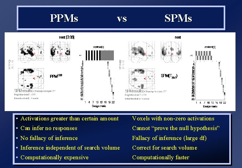
PPMs vs SPMs • Activations greater than certain amount Voxels with non-zero activations • Can infer no responses Cannot “prove the null hypothesis” • No fallacy of inference Fallacy of inference (large df) • Inference independent of search volume Correct for search volume • Computationally expensive Computationally faster

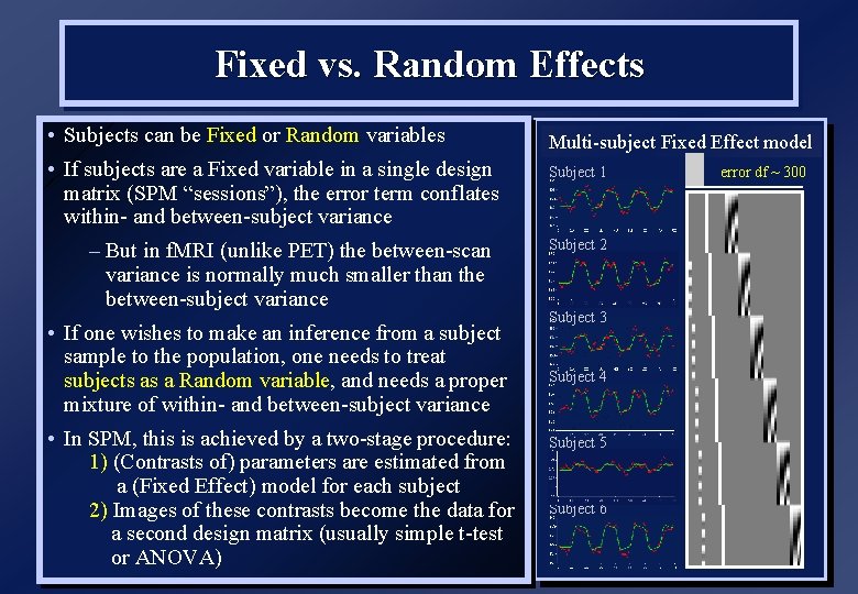
Fixed vs. Random Effects • Subjects can be Fixed or Random variables • If subjects are a Fixed variable in a single design matrix (SPM “sessions”), the error term conflates within- and between-subject variance – But in f. MRI (unlike PET) the between-scan variance is normally much smaller than the between-subject variance • If one wishes to make an inference from a subject sample to the population, one needs to treat subjects as a Random variable, and needs a proper mixture of within- and between-subject variance • In SPM, this is achieved by a two-stage procedure: 1) (Contrasts of) parameters are estimated from a (Fixed Effect) model for each subject 2) Images of these contrasts become the data for a second design matrix (usually simple t-test or ANOVA) Multi-subject Fixed Effect model Subject 1 Subject 2 Subject 3 Subject 4 Subject 5 Subject 6 error df ~ 300

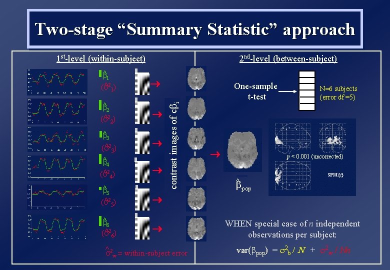
Two-stage “Summary Statistic” approach 2 nd-level (between-subject) 1 st-level (within-subject) b^2 ( ^ 2) b^3 ( ^ 3) b^4 ( ^ 4) b^5 ( ^ 5) b^6 ( ^ 6) One-sample t-test contrast images of cbi b^1 ( ^ 1) ^ = within-subject error w N=6 subjects (error df =5) p < 0. 001 (uncorrected) ^ b pop SPM{t} WHEN special case of n independent observations per subject: var(bpop) = 2 b / N + 2 w / Nn

Limitations of 2 -stage approach • Summary statistic approach is a special case, valid only when each subject’s design matrix is identical (“balanced designs”), and underlyng error identical • In practice, the approach is reasonably robust to unbalanced designs (Penny, 2004) • More generally, exact solutions (“mixed effects”) can be obtained using hierarchical GLM and EM • This is computationally expensive to perform at every voxel (so not implemented in SPM…) • …plus modelling of nonsphericity at 2 nd-level can minimise potential bias of unbalanced designs

The End