Statistical NLP Winter 2008 Language models part II

Statistical NLP Winter 2008 Language models, part II: smoothing Roger Levy thanks to Dan Klein and Jason Eisner

Recap: Language Models • Why are language models useful? • Samples of generated text • What are the main challenges in building n-gram language models? • Discounting versus Backoff/Interpolation

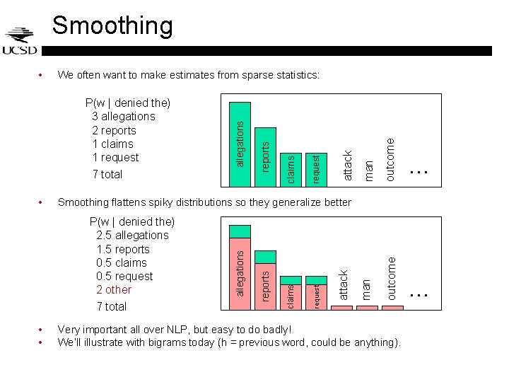
Smoothing man outcome attack request claims reports P(w | denied the) 2. 5 allegations 1. 5 reports 0. 5 claims 0. 5 request 2 other 7 total • • … … Smoothing flattens spiky distributions so they generalize better allegations • request 7 total claims P(w | denied the) 3 allegations 2 reports 1 claims 1 request reports We often want to make estimates from sparse statistics: allegations • Very important all over NLP, but easy to do badly! We’ll illustrate with bigrams today (h = previous word, could be anything).

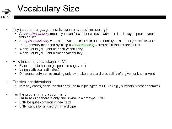
Vocabulary Size • Key issue for language models: open or closed vocabulary? • A closed vocabulary means you can fix a set of words in advanced that may appear in your training set • An open vocabulary means that you need to hold out probability mass for any possible word • Generally managed by fixing a vocabulary list; words not in this list are OOVs • When would you want an open vocabulary? • When would you want a closed vocabulary? • How to set the vocabulary size V? • By external factors (e. g. speech recognizers) • Using statistical estimates? • Difference between estimating unknown token rate and probability of a given unknown word • Practical considerations • In many cases, open vocabularies use multiple types of OOVs (e. g. , numbers & proper names) • For the programming assignment: • OK to assume there is only one unknown word type, UNK • UNK be quite common in new text! • UNK stands for all unknown word type

Five types of smoothing • Today we’ll cover • • • Add- smoothing (Laplace) Simple interpolation Good-Turing smoothing Katz smoothing Kneser-Ney smoothing

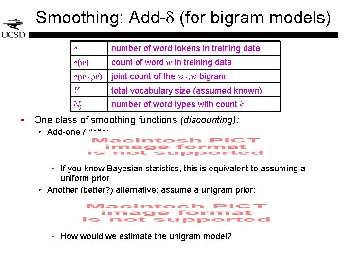
Smoothing: Add- (for bigram models) c number of word tokens in training data c(w) count of word w in training data c(w-1, w) joint count of the w-1, w bigram V total vocabulary size (assumed known) Nk number of word types with count k • One class of smoothing functions (discounting): • Add-one / delta: • If you know Bayesian statistics, this is equivalent to assuming a uniform prior • Another (better? ) alternative: assume a unigram prior: • How would we estimate the unigram model?

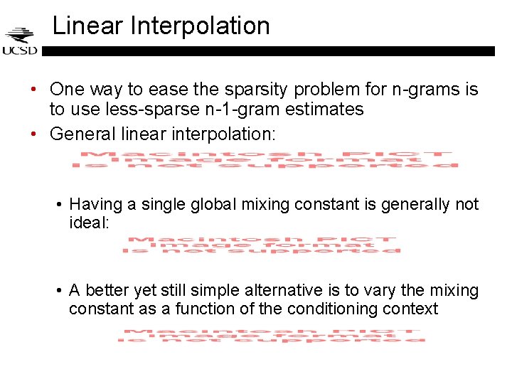
Linear Interpolation • One way to ease the sparsity problem for n-grams is to use less-sparse n-1 -gram estimates • General linear interpolation: • Having a single global mixing constant is generally not ideal: • A better yet still simple alternative is to vary the mixing constant as a function of the conditioning context

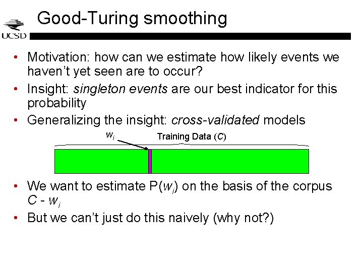
Good-Turing smoothing • Motivation: how can we estimate how likely events we haven’t yet seen are to occur? • Insight: singleton events are our best indicator for this probability • Generalizing the insight: cross-validated models wi Training Data (C) • We want to estimate P(wi) on the basis of the corpus C - wi • But we can’t just do this naively (why not? )

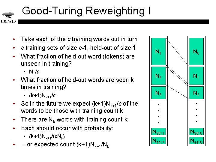
• N 1/c • What fraction of held-out words are seen k times in training? • (k+1)Nk+1/c • So in the future we expect (k+1)Nk+1/c of the words to be those with training count k • There are Nk words with training count k • Each should occur with probability: • (k+1)Nk+1/(c. Nk) • …or expected count (k+1)Nk+1/Nk N 1 N 0 N 2 N 1 N 3 N 2 . . • Take each of the c training words out in turn • c training sets of size c-1, held-out of size 1 • What fraction of held-out word (tokens) are unseen in training? . . Good-Turing Reweighting I N 3511 N 3510 N 4417 N 4416

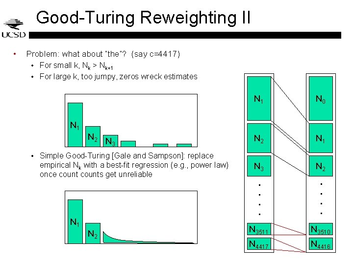
Good-Turing Reweighting II N 1 N 0 N 2 N 1 N 3 N 2 . . Problem: what about “the”? (say c=4417) • For small k, Nk > Nk+1 • For large k, too jumpy, zeros wreck estimates . . • N 1 N 2 N 3 • Simple Good-Turing [Gale and Sampson]: replace empirical Nk with a best-fit regression (e. g. , power law) once counts get unreliable N 1 N 2 N 3511 N 3510 N 4417 N 4416

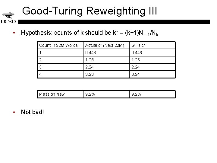
Good-Turing Reweighting III • Hypothesis: counts of k should be k* = (k+1)Nk+1/Nk Count in 22 M Words Actual c* (Next 22 M) GT’s c* 1 0. 448 0. 446 2 1. 25 1. 26 3 2. 24 4 3. 23 3. 24 Mass on New 9. 2% • Not bad!

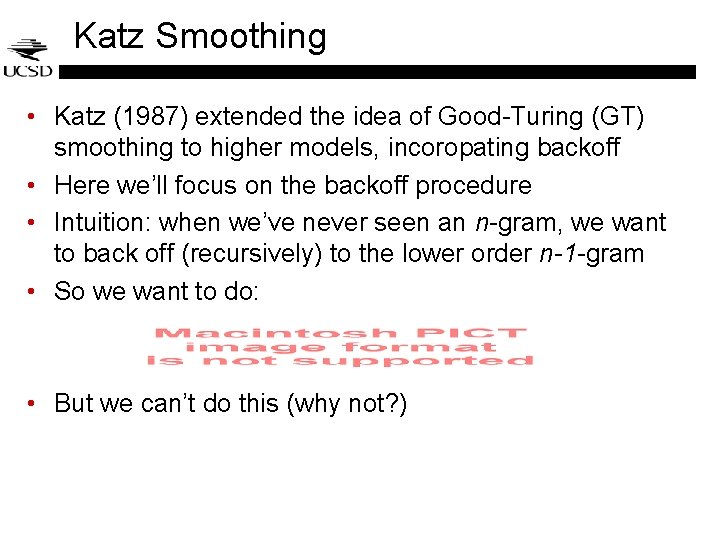
Katz Smoothing • Katz (1987) extended the idea of Good-Turing (GT) smoothing to higher models, incoropating backoff • Here we’ll focus on the backoff procedure • Intuition: when we’ve never seen an n-gram, we want to back off (recursively) to the lower order n-1 -gram • So we want to do: • But we can’t do this (why not? )

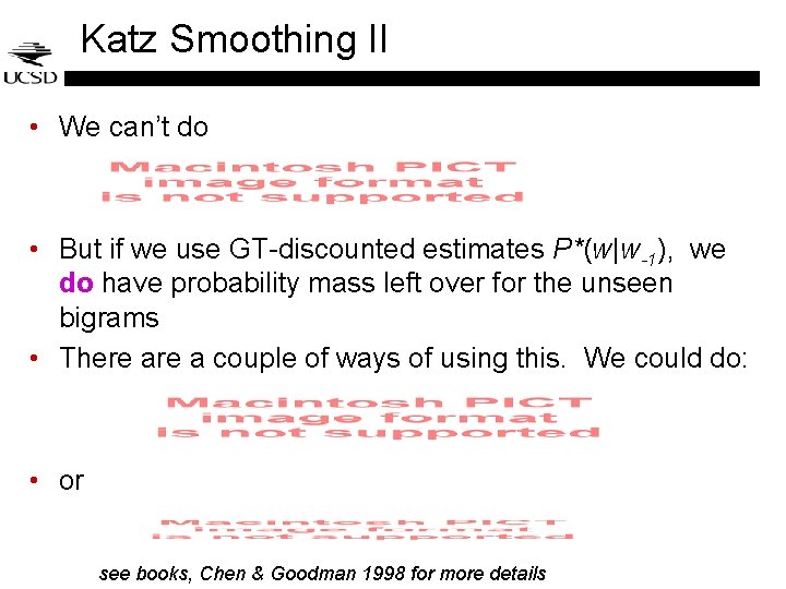
Katz Smoothing II • We can’t do • But if we use GT-discounted estimates P*(w|w-1), we do have probability mass left over for the unseen bigrams • There a couple of ways of using this. We could do: • or see books, Chen & Goodman 1998 for more details

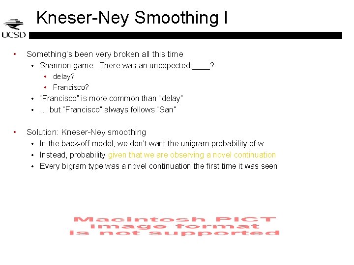
Kneser-Ney Smoothing I • Something’s been very broken all this time • Shannon game: There was an unexpected ____? • delay? • Francisco? • “Francisco” is more common than “delay” • … but “Francisco” always follows “San” • Solution: Kneser-Ney smoothing • In the back-off model, we don’t want the unigram probability of w • Instead, probability given that we are observing a novel continuation • Every bigram type was a novel continuation the first time it was seen

Kneser-Ney Smoothing II • One more aspect to Kneser-Ney: Absolute discounting • Save ourselves some time and just subtract 0. 75 (or some d) • Maybe have a separate value of d for very low counts • More on the board

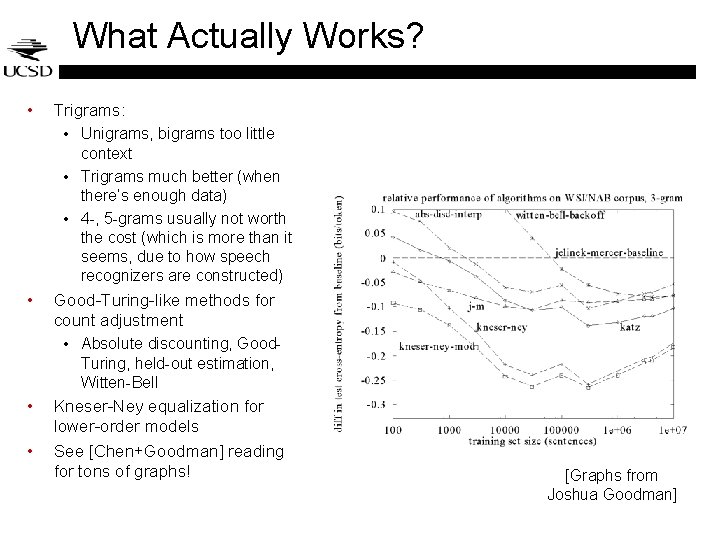
What Actually Works? • Trigrams: • Unigrams, bigrams too little context • Trigrams much better (when there’s enough data) • 4 -, 5 -grams usually not worth the cost (which is more than it seems, due to how speech recognizers are constructed) • Good-Turing-like methods for count adjustment • Absolute discounting, Good. Turing, held-out estimation, Witten-Bell • • Kneser-Ney equalization for lower-order models See [Chen+Goodman] reading for tons of graphs! [Graphs from Joshua Goodman]

Data >> Method? • Having more data is always good… • … but so is picking a better smoothing mechanism! • N > 3 often not worth the cost (greater than you’d think)

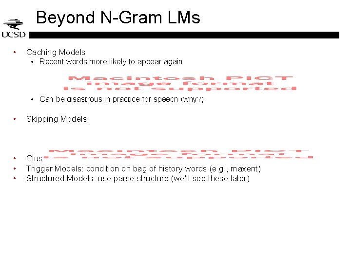
Beyond N-Gram LMs • Caching Models • Recent words more likely to appear again • Can be disastrous in practice for speech (why? ) • Skipping Models • • • Clustering Models: condition on word classes when words are too sparse Trigger Models: condition on bag of history words (e. g. , maxent) Structured Models: use parse structure (we’ll see these later)