Statistical Modeling and Data Analysis Given a data

Population of cancer patients with a probability distribution Population of normal patients with a

The same can be said about weather map. 11

Data Analysis Generally speaking, we perform one or more of the following tasks in

Sample …… -- -- observed observed …… -- -- 14

normal cancer Systolic blood pressure 19

Computation of the posterior There are two popular techniques of computing posterior distribution: 1.

Frequentist vs. Bayesian Frequentist Bayesian All data information is contained in the likelihood function.

Analysis of Variance (ANOVA) ANOVA is one of the most popular statistical tools of

Example 1: You are doing a research on mpg (miles per gallon) for a

Example 2: Research Question: Does blood pressure (BP) depend on weight and gender? Weight

There is a variation in BP. Some is due to weight, and some is

Multiple Hypotheses: Consider 1000 independent tests each at Type-error of α = 0. 05.

If m is large, α would be very small. Thus the power of detecting

Simes Method (Biometrika, 1986): • If , reject all nulls. • If not, but

False Discovery Rate (FDR): Benjamini and Hochberg (1995), JRSS When the number of hypotheses

FDR = Expected proportion of false rejections. Accept Null Reject Null True Null U

Benjamini and Hochberg proved that the following procedure produces : Let k be the

Bayesian Interpretation (Storey, 2003, Ann. Stat. ) are independently distributed. Note: p. FDR is

Directional Hypothesis Problem (Three decision problem): Suppose is rejected, but it is also important

Example: Gene selection When the genes are altered under adverse condition, such as cancer,

Directional Error (Type III error): Type III error is defined as P( Selection of

Slides: 57

Download presentation

Statistical Modeling and Data Analysis Given a data set, first question a statistician ask is, “What is the statistical model to this data? ” We then characterize and analyze the parameters of the model with an objective in mind. • Example : SBP of Cancer Patients vs. Normal patients Cancer: 145, 165, 134, 120, 112, 156, 145, 133, 135, 120 Normal: 138, 120, 112, 110, 128, 134, 128, 109, 138, 140 Objective: Do cancer patients have higher SBP than the normal patients? 1

Population of cancer patients with a probability distribution Population of normal patients with a probability distribution normal cancer Systolic blood pressure Does the data support this hypothesis? 2

Image Process: 9

The same can be said about weather map. 11

Data Analysis Generally speaking, we perform one or more of the following tasks in data analysis (statistical inference) • Estimate the model • Hypothesis testing • Predictive analysis Given the sample data, objective is to make inference about the population described by the probability model. All inferences are based on probability model assumed. 12

Sample …… -- -- observed observed …… -- -- 14

normal cancer Systolic blood pressure 19

Computation of the posterior There are two popular techniques of computing posterior distribution: 1. Metropolis-Hasting Algorithm 2. Gibbs Sampler These techniques can be used effectively for complex probability model and reasonable priors. 24

Frequentist vs. Bayesian Frequentist Bayesian All data information is contained in the likelihood function. All data information is contained in the likelihood function and the prior The estimates are viewed in terms of how they behave on the average Estimates are viewed in terms of where they are located in the posterior Estimates are generally obtained by maximizing the likelihood function. Techniques include Newton-Raphson, EM-algorithm Estimates are obtained from the posterior. Techniques include Gibbas Sampler, Metropolis-Hasting etc. 25

Analysis of Variance (ANOVA) ANOVA is one of the most popular statistical tools of analyzing data. Factor 1 Y Factor 2 A Response Variable Factor 3 Does Y (the response) depends on any of the factors? 29

Example 1: You are doing a research on mpg (miles per gallon) for a brand of automobiles. Question: What effects mpg? Wind speed mpg Air temperature Air moisture Do wind speed, air temperature, and air moisture effect mpg? 30

Example 2: Research Question: Does blood pressure (BP) depend on weight and gender? Weight BP Gender 31

There is a variation in BP. Some is due to weight, and some is due to gender. BP * Female * Male * ** * * * * Weight 32

Multiple Hypotheses: Consider 1000 independent tests each at Type-error of α = 0. 05. Then 5% of the null hypotheses would be falsely rejected. In other words, if 50 of the hypotheses were rejected, there is no guarantee that they were not all falsely rejected. FWER: m = # of hypotheses π = P(One or more falsely rejected hypotheses) = 1 – (Bonferroni Correction)

If m is large, α would be very small. Thus the power of detecting any true positive would be very small. Sequential Bonferroni Corrections: Let be the p-values of independent tests with corresponding null hypotheses . Holm’s Method (Holm, 1979; Scand. Statist. ) • If , accept all nulls. • If , reject ; if , accept the rest of nulls. • Continue until first j such that . In that case reject all and accept the rest of nulls.

Simes Method (Biometrika, 1986): • If , reject all nulls. • If not, but if , reject all • Continue until first . In that case reject all Note: Both Holm’s and Simes methods are designed to refine the FWER.

False Discovery Rate (FDR): Benjamini and Hochberg (1995), JRSS When the number of hypotheses m is very large (say in thousands), and if each individual hypothesis is not important, then FWER criterion is not very useful since it yields few discoveries. For example, in a microarray data analysis, the objective is to detect potential genes for future exploration. Here, each individual gene is not important. In such cases, tests with a controlled FWER would yield few discoveries.

FDR = Expected proportion of false rejections. Accept Null Reject Null True Null U V True Alternatives T S m- R R FDR = = Note that FWER = P(R>0) Total m

Benjamini and Hochberg proved that the following procedure produces : Let k be the largest integer i such that , then reject all The result was proved under the assumption of independent test statistics. It was later extended to a positively correlated test statistics by Benjamini and Yekutieli, 2001; Ann. Stat.

Bayesian Interpretation (Storey, 2003, Ann. Stat. ) are independently distributed. Note: p. FDR is a posterior version of the Type-I error

Directional Hypothesis Problem (Three decision problem): Suppose is rejected, but it is also important to find the direction of So the problem is to find subsets

Example: Gene selection When the genes are altered under adverse condition, such as cancer, the affected genes show under or over expression in a microarray. The objective is to find the genes with under expressions and genes with over expressions.

Directional Error (Type III error): Type III error is defined as P( Selection of false direction if the null is rejected). The traditional method does not control the directional error. For example, Sarkar and Zhou (2008, JSPI) Finner ( 1999, AS) Shaffer (2002, Psychological Methods) Lehmann (1952, AMS; 1957, AMS) Main points of these work is that if the objective is to find the true direction of the alternative after rejecting the null, then a Type III error must be controlled instead of Type I error.

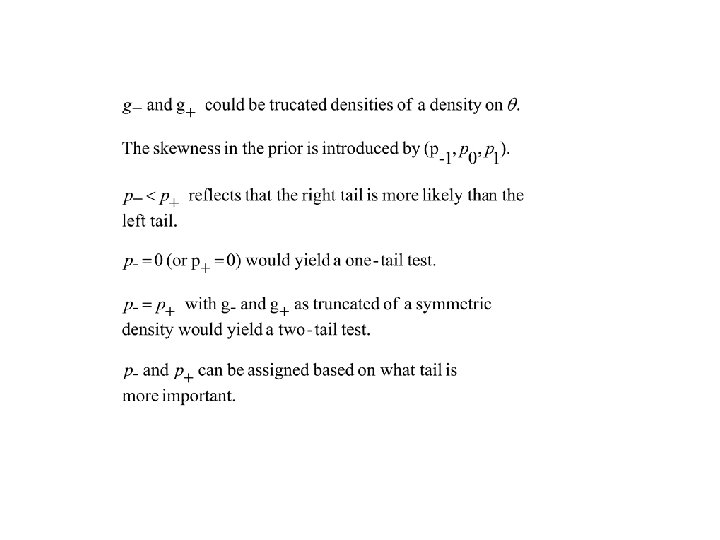
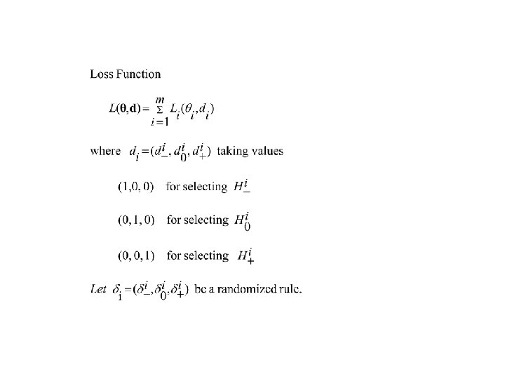
Bayesian Decision Theoretic Framework

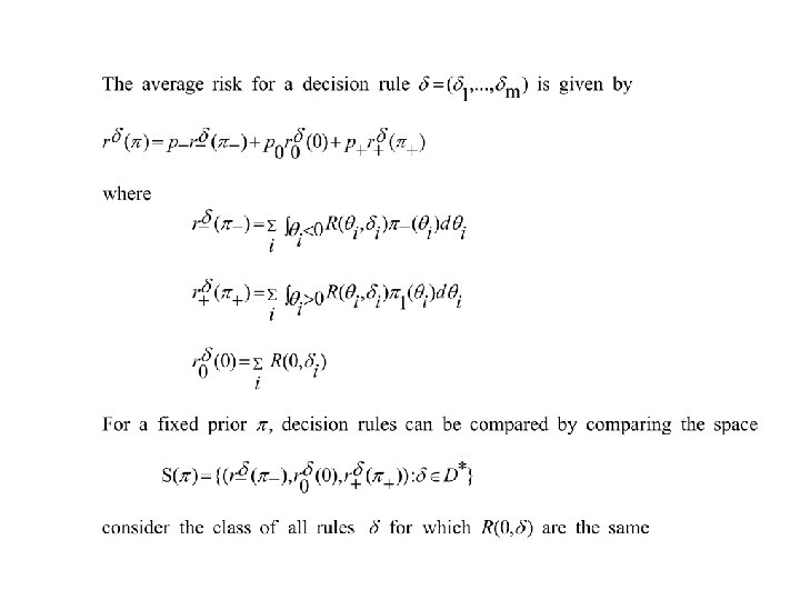
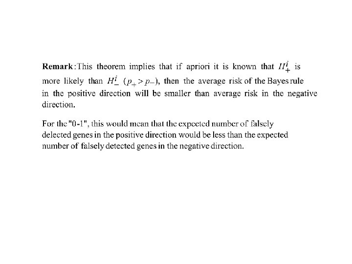
Bayes Rule