Statistical Methods Parameter Estimation https agenda infn itconference

Statistical Methods: Parameter Estimation https: //agenda. infn. it/conference. Display. py? conf. Id=12288 INFN School of Statistics Ischia, 7 -10 May 2017 Glen Cowan Physics Department Royal Holloway, University of London g. cowan@rhul. ac. uk www. pp. rhul. ac. uk/~cowan G. Cowan INFN School of Statistics, Ischia, 7 -10 May 2017 1

Rough outline I. Basic ideas of parameter estimation II. The method of Maximum Likelihood (ML) Variance of ML estimators Extended ML III. Method of Least Squares (LS) IV. Bayesian parameter estimation V. Goodness of fit from the likelihood ratio VI. Examples of frequentist and Bayesian approaches VII. Unfolding G. Cowan INFN School of Statistics, Ischia, 7 -10 May 2017 2

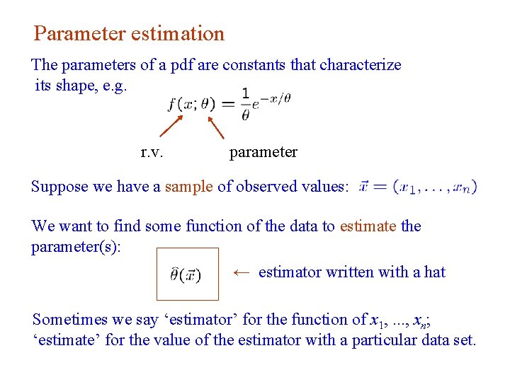
Parameter estimation The parameters of a pdf are constants that characterize its shape, e. g. r. v. parameter Suppose we have a sample of observed values: We want to find some function of the data to estimate the parameter(s): ← estimator written with a hat Sometimes we say ‘estimator’ for the function of x 1, . . . , xn; ‘estimate’ for the value of the estimator with a particular data set. G. Cowan INFN School of Statistics, Ischia, 7 -10 May 2017 3

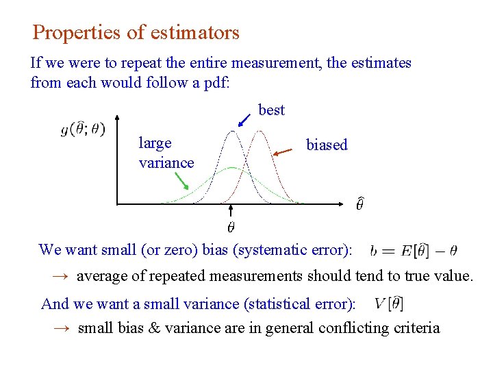
Properties of estimators If we were to repeat the entire measurement, the estimates from each would follow a pdf: best large variance biased We want small (or zero) bias (systematic error): → average of repeated measurements should tend to true value. And we want a small variance (statistical error): → small bias & variance are in general conflicting criteria G. Cowan INFN School of Statistics, Ischia, 7 -10 May 2017 4

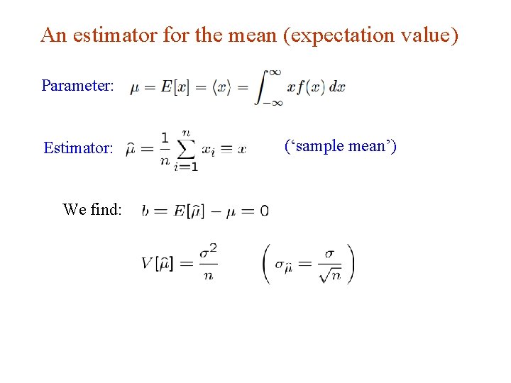
An estimator for the mean (expectation value) Parameter: Estimator: (‘sample mean’) We find: G. Cowan INFN School of Statistics, Ischia, 7 -10 May 2017 5

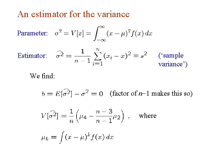
An estimator for the variance Parameter: (‘sample variance’) Estimator: We find: (factor of n-1 makes this so) where G. Cowan INFN School of Statistics, Ischia, 7 -10 May 2017 6

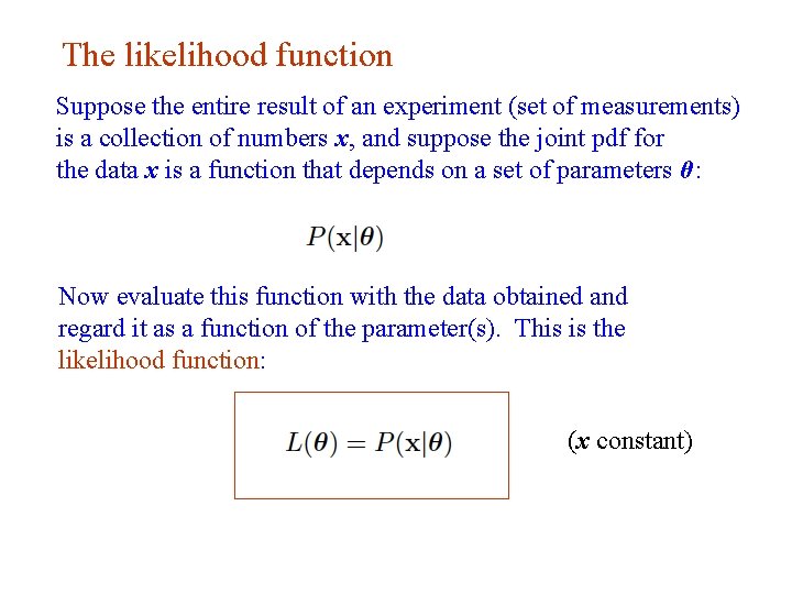
The likelihood function Suppose the entire result of an experiment (set of measurements) is a collection of numbers x, and suppose the joint pdf for the data x is a function that depends on a set of parameters θ: Now evaluate this function with the data obtained and regard it as a function of the parameter(s). This is the likelihood function: (x constant) G. Cowan INFN School of Statistics, Ischia, 7 -10 May 2017 7

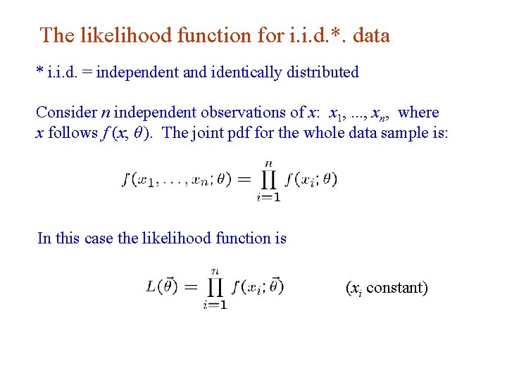
The likelihood function for i. i. d. *. data * i. i. d. = independent and identically distributed Consider n independent observations of x: x 1, . . . , xn, where x follows f (x; θ ). The joint pdf for the whole data sample is: In this case the likelihood function is (xi constant) G. Cowan INFN School of Statistics, Ischia, 7 -10 May 2017 8

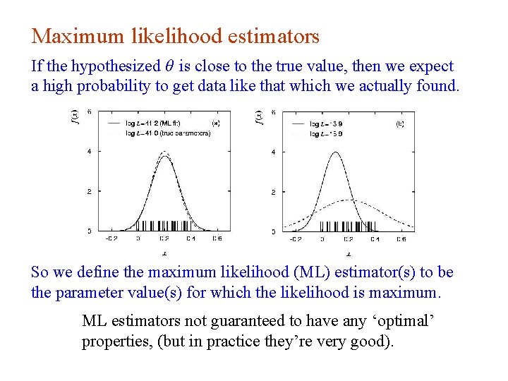
Maximum likelihood estimators If the hypothesized θ is close to the true value, then we expect a high probability to get data like that which we actually found. So we define the maximum likelihood (ML) estimator(s) to be the parameter value(s) for which the likelihood is maximum. ML estimators not guaranteed to have any ‘optimal’ properties, (but in practice they’re very good). G. Cowan INFN School of Statistics, Ischia, 7 -10 May 2017 9

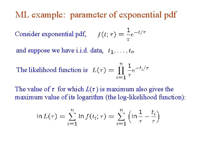
ML example: parameter of exponential pdf Consider exponential pdf, and suppose we have i. i. d. data, The likelihood function is The value of τ for which L(τ ) is maximum also gives the maximum value of its logarithm (the log-likelihood function): G. Cowan INFN School of Statistics, Ischia, 7 -10 May 2017 10

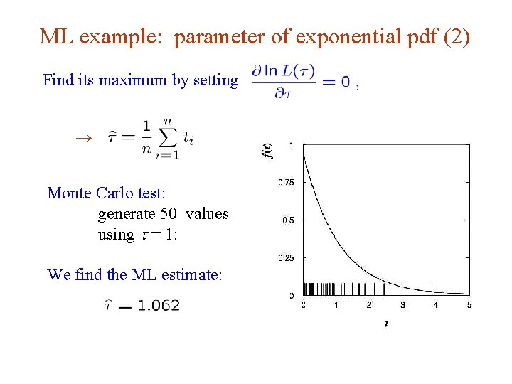
ML example: parameter of exponential pdf (2) Find its maximum by setting → Monte Carlo test: generate 50 values using t = 1: We find the ML estimate: G. Cowan INFN School of Statistics, Ischia, 7 -10 May 2017 11

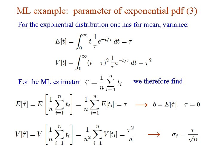
ML example: parameter of exponential pdf (3) For the exponential distribution one has for mean, variance: For the ML estimator we therefore find → → G. Cowan INFN School of Statistics, Ischia, 7 -10 May 2017 12

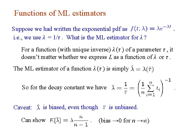
Functions of ML estimators Suppose we had written the exponential pdf as i. e. , we use λ = 1/τ. What is the ML estimator for λ ? For a function (with unique inverse) λ (τ ) of a parameter τ , it doesn’t matter whether we express L as a function of λ or τ. The ML estimator of a function λ (τ ) is simply So for the decay constant we have Caveat: is biased, even though Can show G. Cowan is unbiased. (bias → 0 for n →∞) INFN School of Statistics, Ischia, 7 -10 May 2017 13

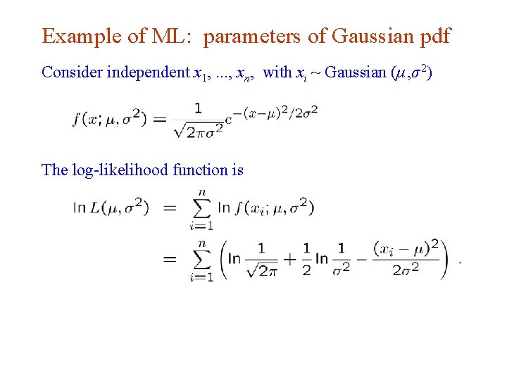
Example of ML: parameters of Gaussian pdf Consider independent x 1, . . . , xn, with xi ~ Gaussian (μ, σ 2) The log-likelihood function is G. Cowan INFN School of Statistics, Ischia, 7 -10 May 2017 14

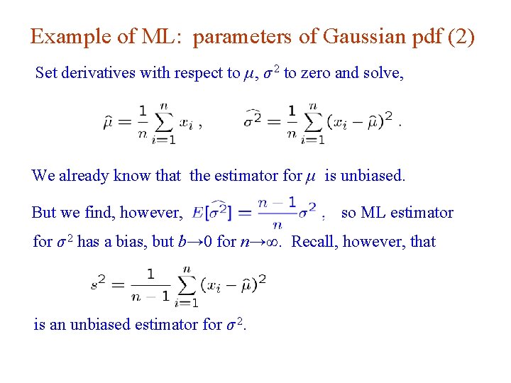
Example of ML: parameters of Gaussian pdf (2) Set derivatives with respect to μ, σ 2 to zero and solve, We already know that the estimator for μ is unbiased. But we find, however, so ML estimator for σ 2 has a bias, but b→ 0 for n→∞. Recall, however, that is an unbiased estimator for σ 2. G. Cowan INFN School of Statistics, Ischia, 7 -10 May 2017 15

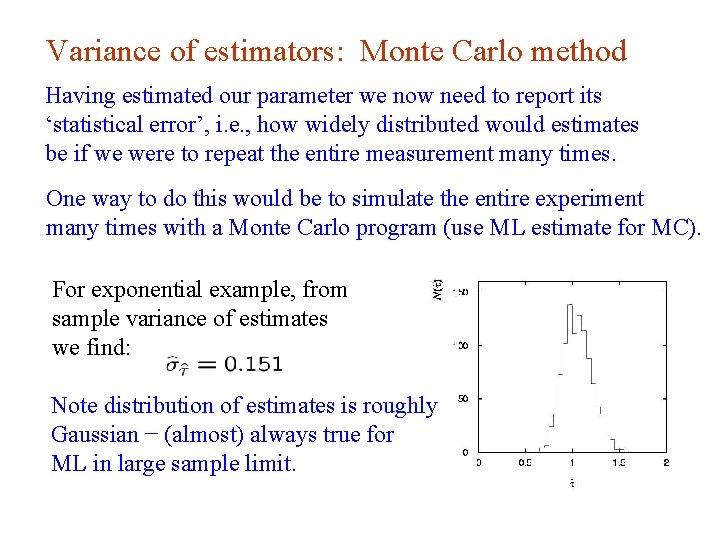
Variance of estimators: Monte Carlo method Having estimated our parameter we now need to report its ‘statistical error’, i. e. , how widely distributed would estimates be if we were to repeat the entire measurement many times. One way to do this would be to simulate the entire experiment many times with a Monte Carlo program (use ML estimate for MC). For exponential example, from sample variance of estimates we find: Note distribution of estimates is roughly Gaussian − (almost) always true for ML in large sample limit. G. Cowan INFN School of Statistics, Ischia, 7 -10 May 2017 16

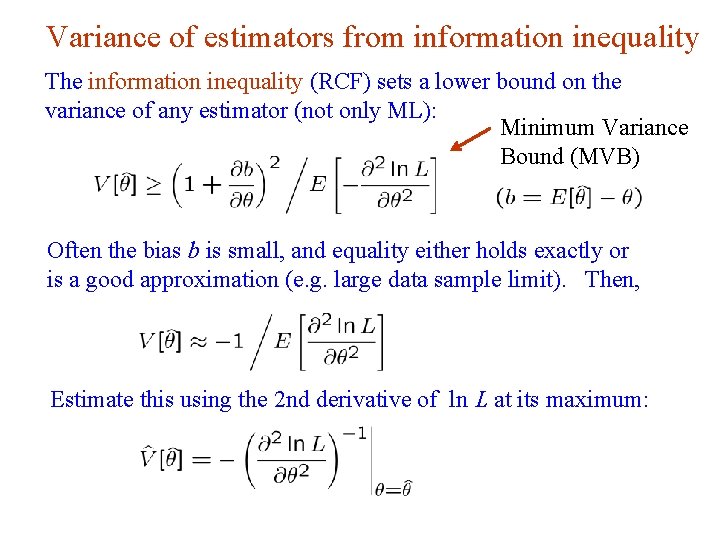
Variance of estimators from information inequality The information inequality (RCF) sets a lower bound on the variance of any estimator (not only ML): Minimum Variance Bound (MVB) Often the bias b is small, and equality either holds exactly or is a good approximation (e. g. large data sample limit). Then, Estimate this using the 2 nd derivative of ln L at its maximum: G. Cowan INFN School of Statistics, Ischia, 7 -10 May 2017 17

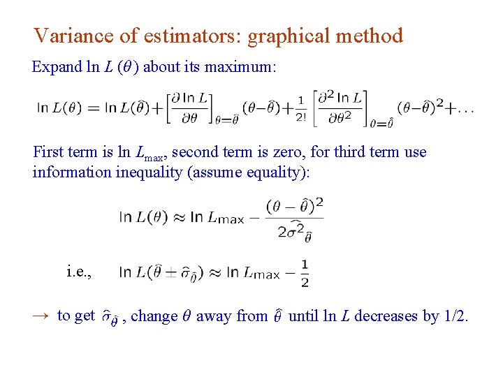
Variance of estimators: graphical method Expand ln L (θ ) about its maximum: First term is ln Lmax, second term is zero, for third term use information inequality (assume equality): i. e. , → to get G. Cowan , change θ away from until ln L decreases by 1/2. INFN School of Statistics, Ischia, 7 -10 May 2017 18

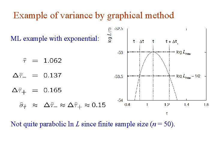
Example of variance by graphical method ML example with exponential: Not quite parabolic ln L since finite sample size (n = 50). G. Cowan INFN School of Statistics, Ischia, 7 -10 May 2017 19

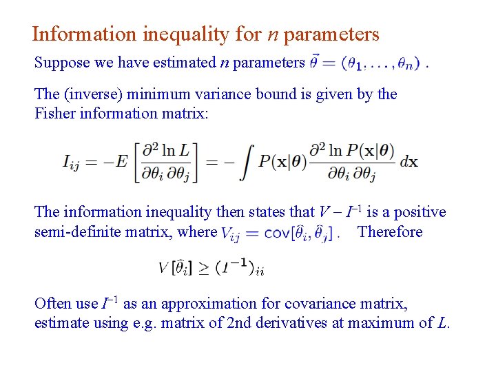
Information inequality for n parameters Suppose we have estimated n parameters The (inverse) minimum variance bound is given by the Fisher information matrix: The information inequality then states that V - I-1 is a positive semi-definite matrix, where Therefore Often use I-1 as an approximation for covariance matrix, estimate using e. g. matrix of 2 nd derivatives at maximum of L. G. Cowan INFN School of Statistics, Ischia, 7 -10 May 2017 20

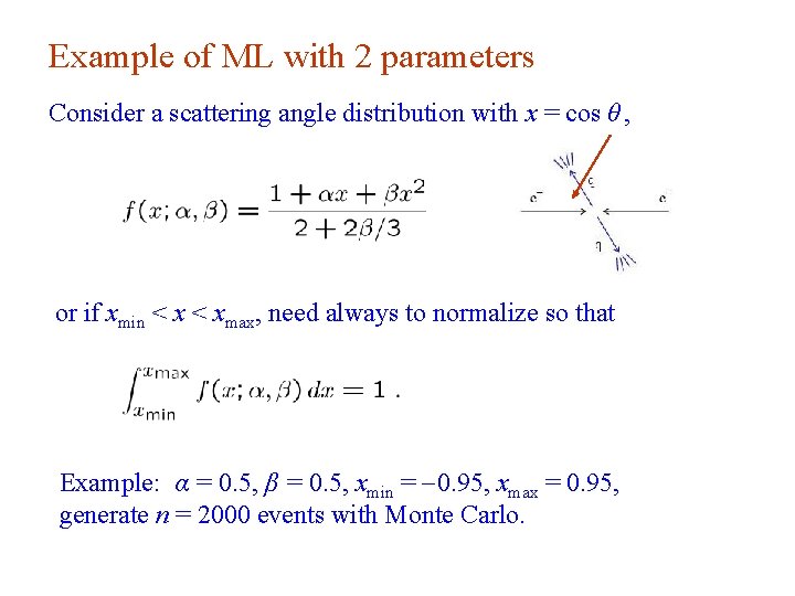
Example of ML with 2 parameters Consider a scattering angle distribution with x = cos θ , or if xmin < xmax, need always to normalize so that Example: α = 0. 5, β = 0. 5, xmin = -0. 95, xmax = 0. 95, generate n = 2000 events with Monte Carlo. G. Cowan INFN School of Statistics, Ischia, 7 -10 May 2017 21

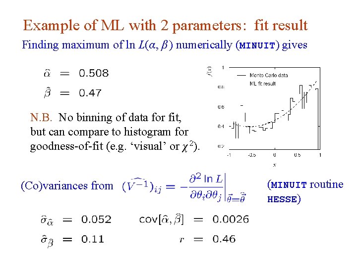
Example of ML with 2 parameters: fit result Finding maximum of ln L(α, β ) numerically (MINUIT) gives N. B. No binning of data for fit, but can compare to histogram for goodness-of-fit (e. g. ‘visual’ or χ 2). (Co)variances from G. Cowan INFN School of Statistics, Ischia, 7 -10 May 2017 (MINUIT routine HESSE) 22

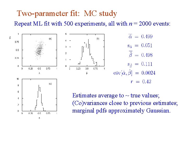
Two-parameter fit: MC study Repeat ML fit with 500 experiments, all with n = 2000 events: Estimates average to ~ true values; (Co)variances close to previous estimates; marginal pdfs approximately Gaussian. G. Cowan INFN School of Statistics, Ischia, 7 -10 May 2017 23

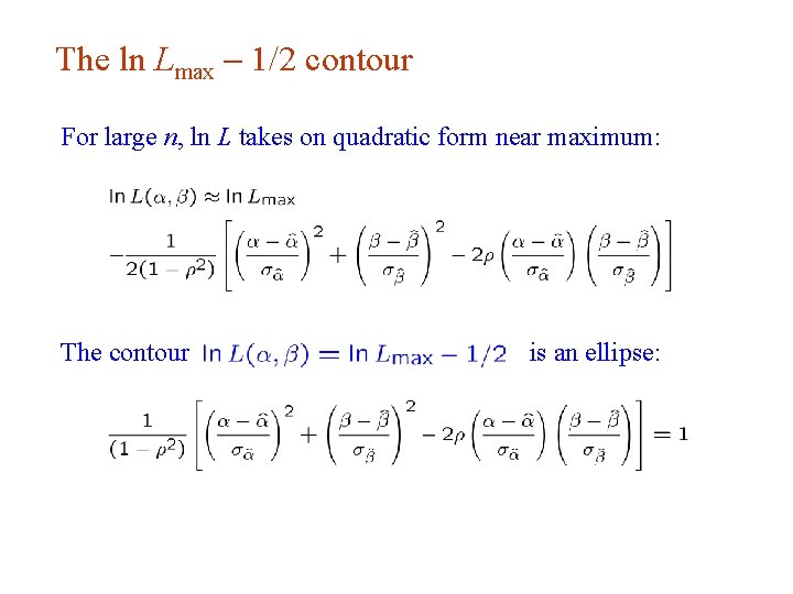
The ln Lmax - 1/2 contour For large n, ln L takes on quadratic form near maximum: The contour G. Cowan is an ellipse: INFN School of Statistics, Ischia, 7 -10 May 2017 24

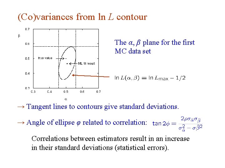
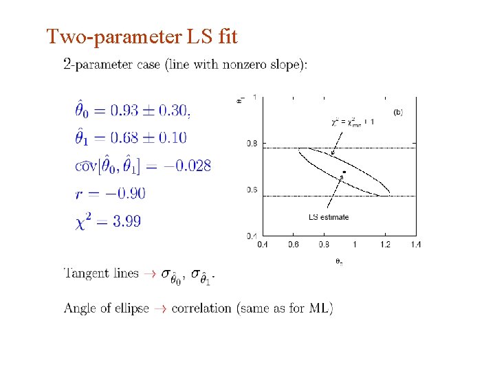
(Co)variances from ln L contour The α, β plane for the first MC data set → Tangent lines to contours give standard deviations. → Angle of ellipse φ related to correlation: Correlations between estimators result in an increase in their standard deviations (statistical errors). G. Cowan INFN School of Statistics, Ischia, 7 -10 May 2017 25

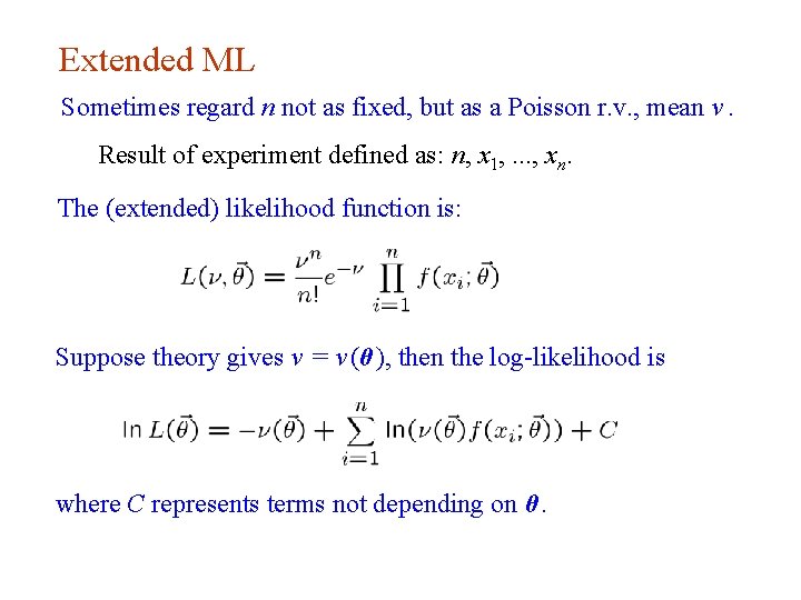
Extended ML Sometimes regard n not as fixed, but as a Poisson r. v. , mean ν. Result of experiment defined as: n, x 1, . . . , xn. The (extended) likelihood function is: Suppose theory gives ν = ν (θ), then the log-likelihood is where C represents terms not depending on θ. G. Cowan INFN School of Statistics, Ischia, 7 -10 May 2017 26

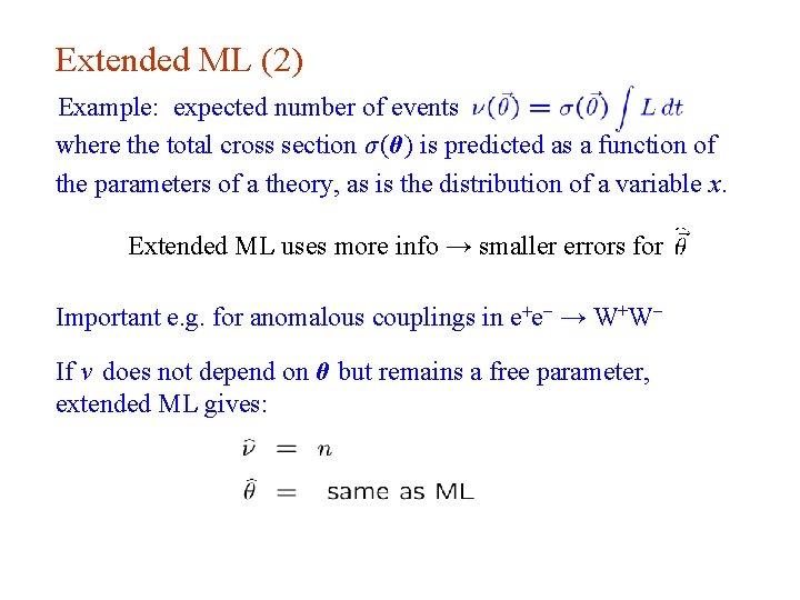
Extended ML (2) Example: expected number of events where the total cross section σ (θ) is predicted as a function of the parameters of a theory, as is the distribution of a variable x. Extended ML uses more info → smaller errors for Important e. g. for anomalous couplings in e+e- → W+WIf ν does not depend on θ but remains a free parameter, extended ML gives: G. Cowan INFN School of Statistics, Ischia, 7 -10 May 2017 27

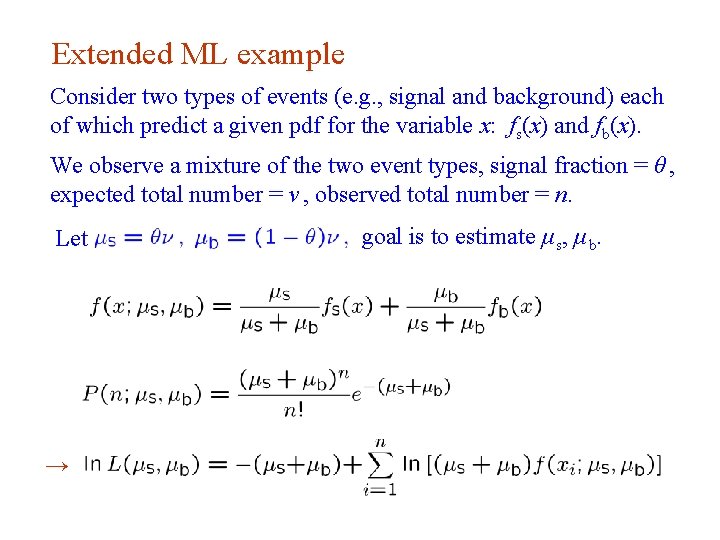
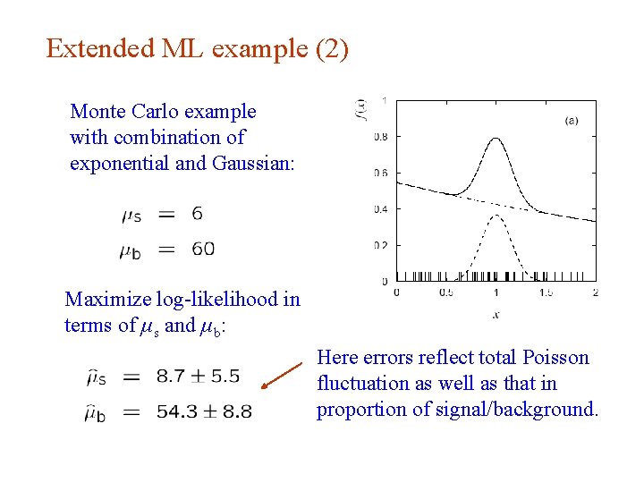
Extended ML example Consider two types of events (e. g. , signal and background) each of which predict a given pdf for the variable x: fs(x) and fb(x). We observe a mixture of the two event types, signal fraction = θ , expected total number = ν , observed total number = n. Let goal is to estimate μ s, μ b. → G. Cowan INFN School of Statistics, Ischia, 7 -10 May 2017 28

Extended ML example (2) Monte Carlo example with combination of exponential and Gaussian: Maximize log-likelihood in terms of μ s and μ b: Here errors reflect total Poisson fluctuation as well as that in proportion of signal/background. G. Cowan INFN School of Statistics, Ischia, 7 -10 May 2017 29

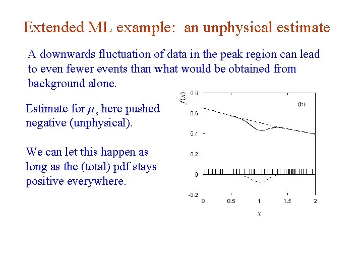
Extended ML example: an unphysical estimate A downwards fluctuation of data in the peak region can lead to even fewer events than what would be obtained from background alone. Estimate for μ s here pushed negative (unphysical). We can let this happen as long as the (total) pdf stays positive everywhere. G. Cowan INFN School of Statistics, Ischia, 7 -10 May 2017 30

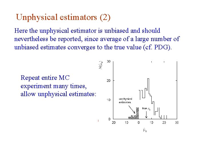
Unphysical estimators (2) Here the unphysical estimator is unbiased and should nevertheless be reported, since average of a large number of unbiased estimates converges to the true value (cf. PDG). Repeat entire MC experiment many times, allow unphysical estimates: G. Cowan INFN School of Statistics, Ischia, 7 -10 May 2017 31

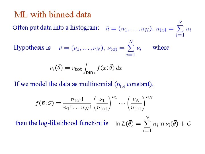
ML with binned data Often put data into a histogram: Hypothesis is where If we model the data as multinomial (ntot constant), then the log-likelihood function is: G. Cowan INFN School of Statistics, Ischia, 7 -10 May 2017 32

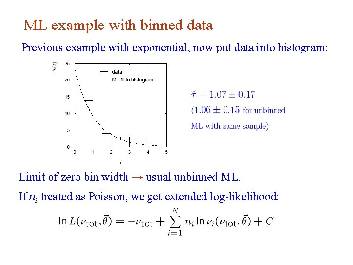
ML example with binned data Previous example with exponential, now put data into histogram: Limit of zero bin width → usual unbinned ML. If ni treated as Poisson, we get extended log-likelihood: G. Cowan INFN School of Statistics, Ischia, 7 -10 May 2017 33

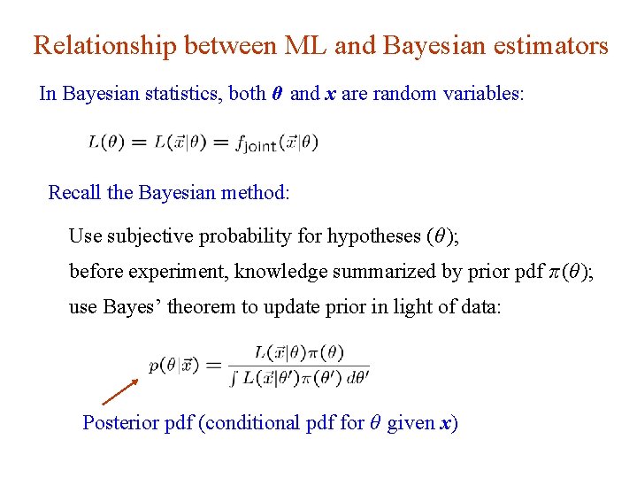
Relationship between ML and Bayesian estimators In Bayesian statistics, both θ and x are random variables: Recall the Bayesian method: Use subjective probability for hypotheses (θ ); before experiment, knowledge summarized by prior pdf π (θ ); use Bayes’ theorem to update prior in light of data: Posterior pdf (conditional pdf for θ given x) G. Cowan INFN School of Statistics, Ischia, 7 -10 May 2017 34

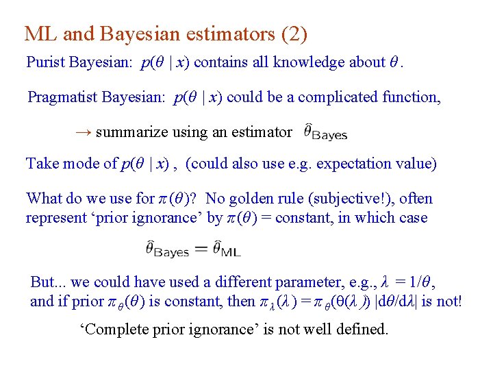
ML and Bayesian estimators (2) Purist Bayesian: p(θ | x) contains all knowledge about θ. Pragmatist Bayesian: p(θ | x) could be a complicated function, → summarize using an estimator Take mode of p(θ | x) , (could also use e. g. expectation value) What do we use for π (θ )? No golden rule (subjective!), often represent ‘prior ignorance’ by π (θ ) = constant, in which case But. . . we could have used a different parameter, e. g. , λ = 1/θ , and if prior π θ (θ ) is constant, then π λ (λ ) = π θ (θ(λ )) |dθ/dλ| is not! ‘Complete prior ignorance’ is not well defined. G. Cowan INFN School of Statistics, Ischia, 7 -10 May 2017 35

Priors from formal rules Because of difficulties in encoding a vague degree of belief in a prior, one often attempts to derive the prior from formal rules, e. g. , to satisfy certain invariance principles or to provide maximum information gain for a certain set of measurements. Often called “objective priors” Form basis of Objective Bayesian Statistics The priors do not reflect a degree of belief (but might represent possible extreme cases). In a Subjective Bayesian analysis, using objective priors can be an important part of the sensitivity analysis. G. Cowan INFN School of Statistics, Ischia, 7 -10 May 2017 36

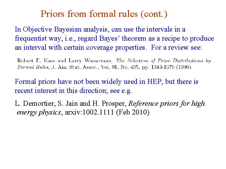
Priors from formal rules (cont. ) In Objective Bayesian analysis, can use the intervals in a frequentist way, i. e. , regard Bayes’ theorem as a recipe to produce an interval with certain coverage properties. For a review see: Formal priors have not been widely used in HEP, but there is recent interest in this direction; see e. g. L. Demortier, S. Jain and H. Prosper, Reference priors for high energy physics, arxiv: 1002. 1111 (Feb 2010) G. Cowan INFN School of Statistics, Ischia, 7 -10 May 2017 37

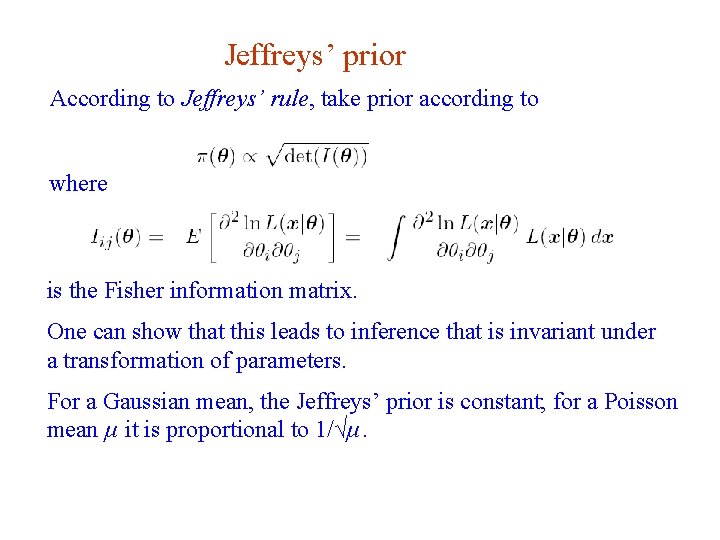
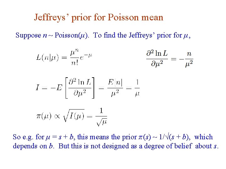
Jeffreys’ prior According to Jeffreys’ rule, take prior according to where is the Fisher information matrix. One can show that this leads to inference that is invariant under a transformation of parameters. For a Gaussian mean, the Jeffreys’ prior is constant; for a Poisson mean μ it is proportional to 1/√μ. G. Cowan INFN School of Statistics, Ischia, 7 -10 May 2017 38

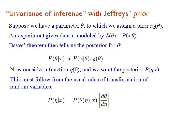
“Invariance of inference” with Jeffreys’ prior Suppose we have a parameter θ, to which we assign a prior πθ(θ). An experiment gives data x, modeled by L(θ) = P(x|θ). Bayes’ theorem then tells us the posterior for θ: Now consider a function η(θ), and we want the posterior P(η|x). This must follow from the usual rules of transformation of random variables: G. Cowan INFN School of Statistics, Ischia, 7 -10 May 2017 39

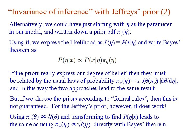
“Invariance of inference” with Jeffreys’ prior (2) Alternatively, we could have just starting with η as the parameter in our model, and written down a prior pdf πη(η). Using it, we express the likelihood as L(η) = P(x|η) and write Bayes’ theorem as If the priors really express our degree of belief, then they must be related by the usual laws of probability π η (η ) = π θ (θ(η )) |dθ/dη|, and in this way the two approaches lead to the same result. But if we choose the priors according to “formal rules”, then this is not guaranteed. For the Jeffrey’s prior, however, it does work! Using πθ(θ) ∝√I(θ) and transforming to find P(η|x) leads to the same as using π η (η ) ∝√I(η ) directly with Bayes’ theorem. G. Cowan INFN School of Statistics, Ischia, 7 -10 May 2017 40

Jeffreys’ prior for Poisson mean Suppose n ~ Poisson(μ). To find the Jeffreys’ prior for μ, So e. g. for μ = s + b, this means the prior π (s) ~ 1/√(s + b), which depends on b. But this is not designed as a degree of belief about s. G. Cowan INFN School of Statistics, Ischia, 7 -10 May 2017 41

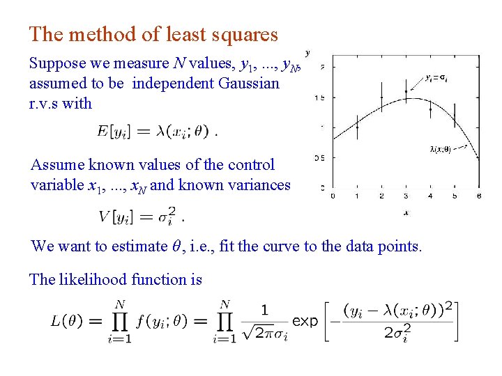
The method of least squares Suppose we measure N values, y 1, . . . , y. N, assumed to be independent Gaussian r. v. s with Assume known values of the control variable x 1, . . . , x. N and known variances We want to estimate θ , i. e. , fit the curve to the data points. The likelihood function is G. Cowan INFN School of Statistics, Ischia, 7 -10 May 2017 42

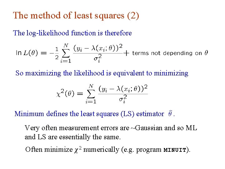
The method of least squares (2) The log-likelihood function is therefore So maximizing the likelihood is equivalent to minimizing Minimum defines the least squares (LS) estimator Very often measurement errors are ~Gaussian and so ML and LS are essentially the same. Often minimize χ 2 numerically (e. g. program MINUIT). G. Cowan INFN School of Statistics, Ischia, 7 -10 May 2017 43

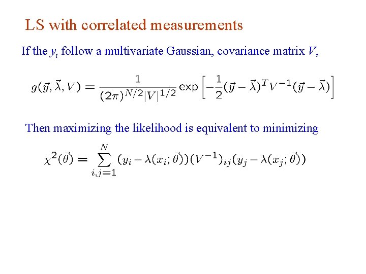
LS with correlated measurements If the yi follow a multivariate Gaussian, covariance matrix V, Then maximizing the likelihood is equivalent to minimizing G. Cowan INFN School of Statistics, Ischia, 7 -10 May 2017 44

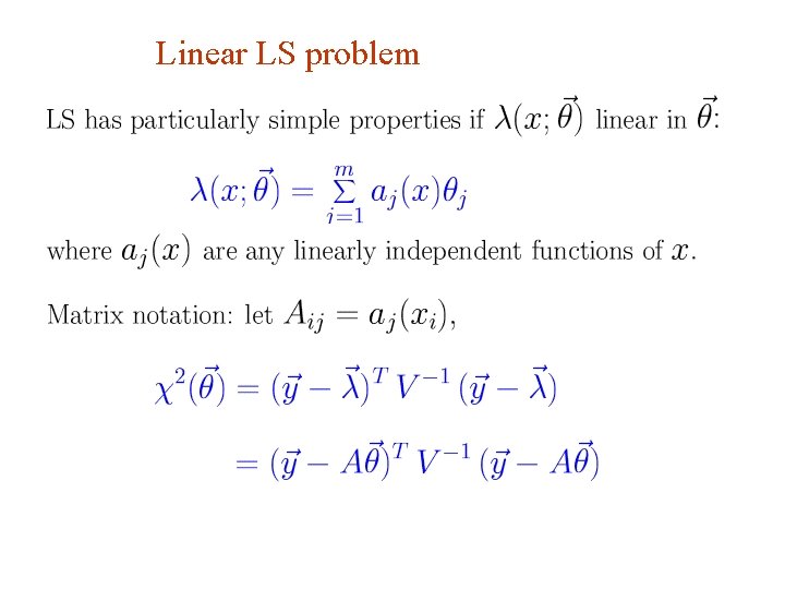
Linear LS problem G. Cowan INFN School of Statistics, Ischia, 7 -10 May 2017 45

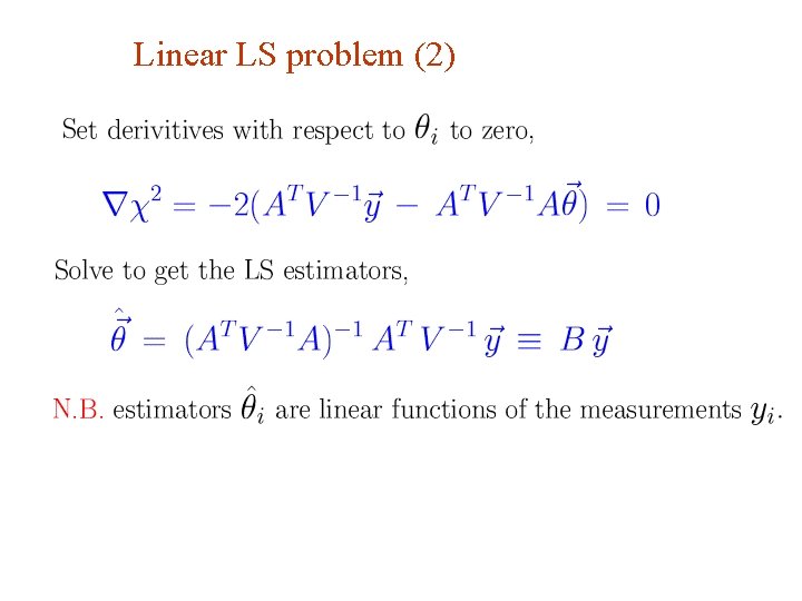
Linear LS problem (2) G. Cowan INFN School of Statistics, Ischia, 7 -10 May 2017 46

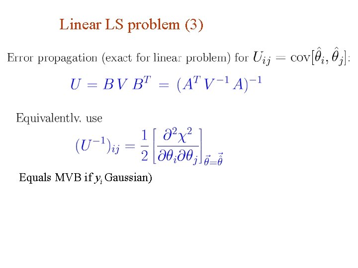
Linear LS problem (3) Equals MVB if yi Gaussian) G. Cowan INFN School of Statistics, Ischia, 7 -10 May 2017 47

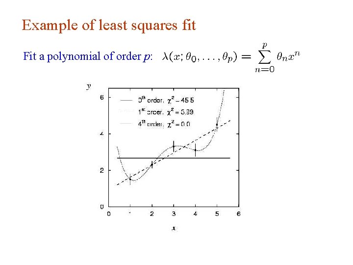
Example of least squares fit Fit a polynomial of order p: G. Cowan INFN School of Statistics, Ischia, 7 -10 May 2017 48

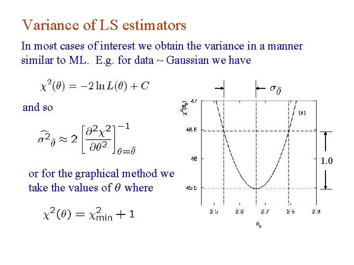
Variance of LS estimators In most cases of interest we obtain the variance in a manner similar to ML. E. g. for data ~ Gaussian we have and so 1. 0 or for the graphical method we take the values of θ where G. Cowan INFN School of Statistics, Ischia, 7 -10 May 2017 49

Two-parameter LS fit G. Cowan INFN School of Statistics, Ischia, 7 -10 May 2017 50

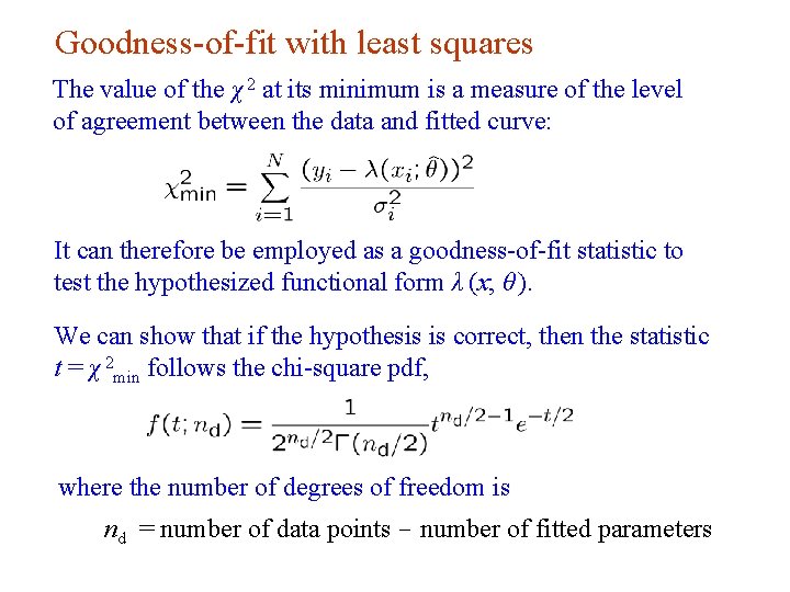
Goodness-of-fit with least squares The value of the χ 2 at its minimum is a measure of the level of agreement between the data and fitted curve: It can therefore be employed as a goodness-of-fit statistic to test the hypothesized functional form λ (x; θ ). We can show that if the hypothesis is correct, then the statistic t = χ 2 min follows the chi-square pdf, where the number of degrees of freedom is nd = number of data points - number of fitted parameters G. Cowan INFN School of Statistics, Ischia, 7 -10 May 2017 51

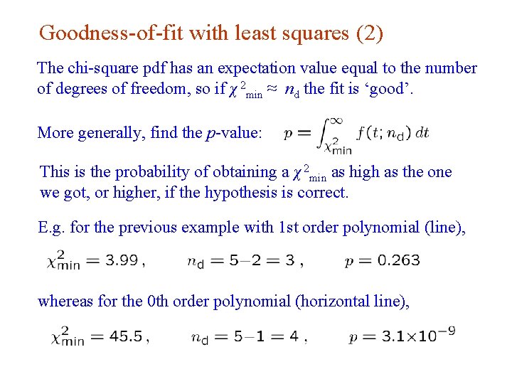
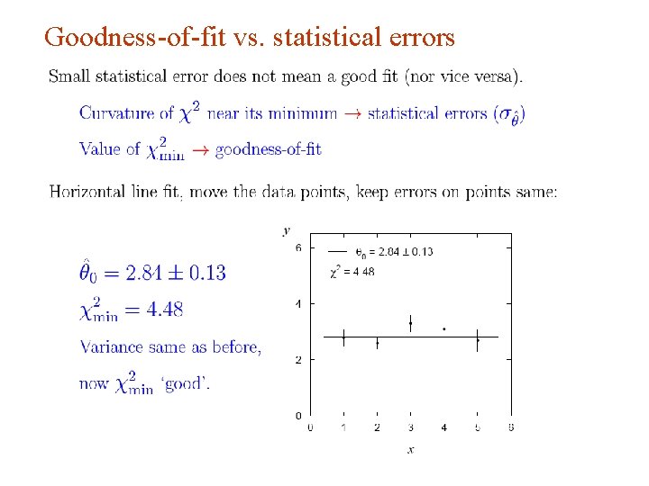
Goodness-of-fit with least squares (2) The chi-square pdf has an expectation value equal to the number of degrees of freedom, so if χ 2 min ≈ nd the fit is ‘good’. More generally, find the p-value: This is the probability of obtaining a χ 2 min as high as the one we got, or higher, if the hypothesis is correct. E. g. for the previous example with 1 st order polynomial (line), whereas for the 0 th order polynomial (horizontal line), G. Cowan INFN School of Statistics, Ischia, 7 -10 May 2017 52

Goodness-of-fit vs. statistical errors G. Cowan INFN School of Statistics, Ischia, 7 -10 May 2017 53

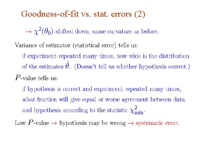
Goodness-of-fit vs. stat. errors (2) G. Cowan INFN School of Statistics, Ischia, 7 -10 May 2017 54

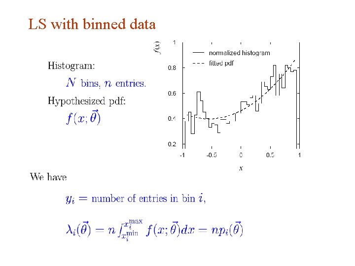
LS with binned data G. Cowan INFN School of Statistics, Ischia, 7 -10 May 2017 55

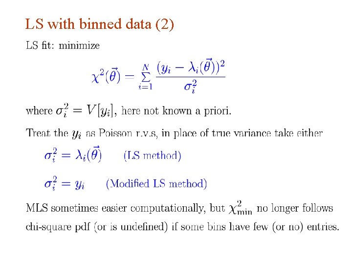
LS with binned data (2) G. Cowan INFN School of Statistics, Ischia, 7 -10 May 2017 56

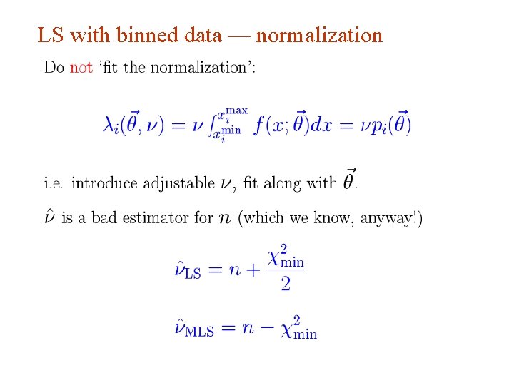
LS with binned data — normalization G. Cowan INFN School of Statistics, Ischia, 7 -10 May 2017 57

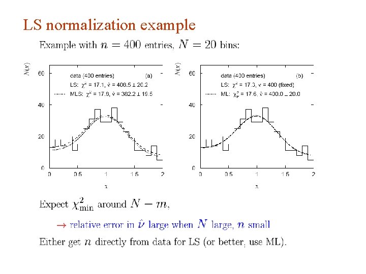
LS normalization example G. Cowan INFN School of Statistics, Ischia, 7 -10 May 2017 58

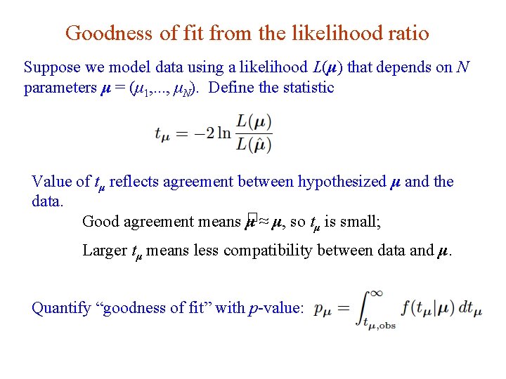
Goodness of fit from the likelihood ratio Suppose we model data using a likelihood L(μ) that depends on N parameters μ = (μ 1, . . . , μΝ). Define the statistic Value of tμ reflects agreement between hypothesized μ and the data. � ≈ μ, so t is small; Good agreement means μ μ Larger tμ means less compatibility between data and μ. Quantify “goodness of fit” with p-value: G. Cowan INFN School of Statistics, Ischia, 7 -10 May 2017 59

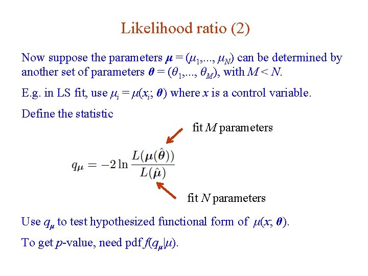
Likelihood ratio (2) Now suppose the parameters μ = (μ 1, . . . , μΝ) can be determined by another set of parameters θ = (θ 1, . . . , θM), with M < N. E. g. in LS fit, use μi = μ(xi; θ) where x is a control variable. Define the statistic fit M parameters fit N parameters Use qμ to test hypothesized functional form of μ(x; θ). To get p-value, need pdf f(qμ|μ). G. Cowan INFN School of Statistics, Ischia, 7 -10 May 2017 60

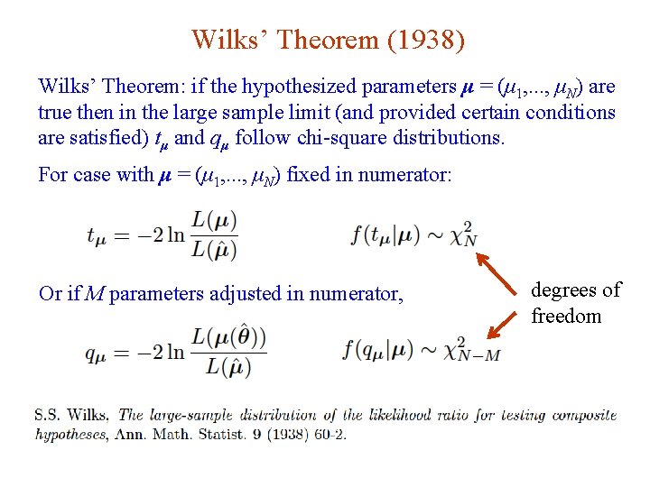
Wilks’ Theorem (1938) Wilks’ Theorem: if the hypothesized parameters μ = (μ 1, . . . , μΝ) are true then in the large sample limit (and provided certain conditions are satisfied) tμ and qμ follow chi-square distributions. For case with μ = (μ 1, . . . , μΝ) fixed in numerator: Or if M parameters adjusted in numerator, G. Cowan INFN School of Statistics, Ischia, 7 -10 May 2017 degrees of freedom 61

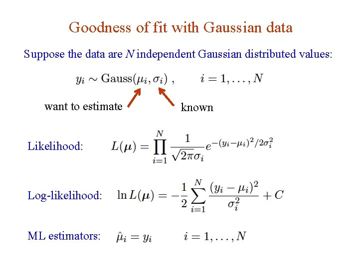
Goodness of fit with Gaussian data Suppose the data are N independent Gaussian distributed values: want to estimate known Likelihood: Log-likelihood: ML estimators: G. Cowan INFN School of Statistics, Ischia, 7 -10 May 2017 62

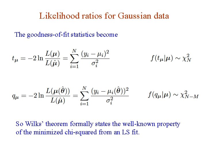
Likelihood ratios for Gaussian data The goodness-of-fit statistics become So Wilks’ theorem formally states the well-known property of the minimized chi-squared from an LS fit. G. Cowan INFN School of Statistics, Ischia, 7 -10 May 2017 63

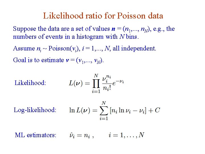
Likelihood ratio for Poisson data Suppose the data are a set of values n = (n 1, . . . , nΝ), e. g. , the numbers of events in a histogram with N bins. Assume ni ~ Poisson(νi), i = 1, . . . , N, all independent. Goal is to estimate ν = (ν 1, . . . , νΝ). Likelihood: Log-likelihood: ML estimators: G. Cowan INFN School of Statistics, Ischia, 7 -10 May 2017 64

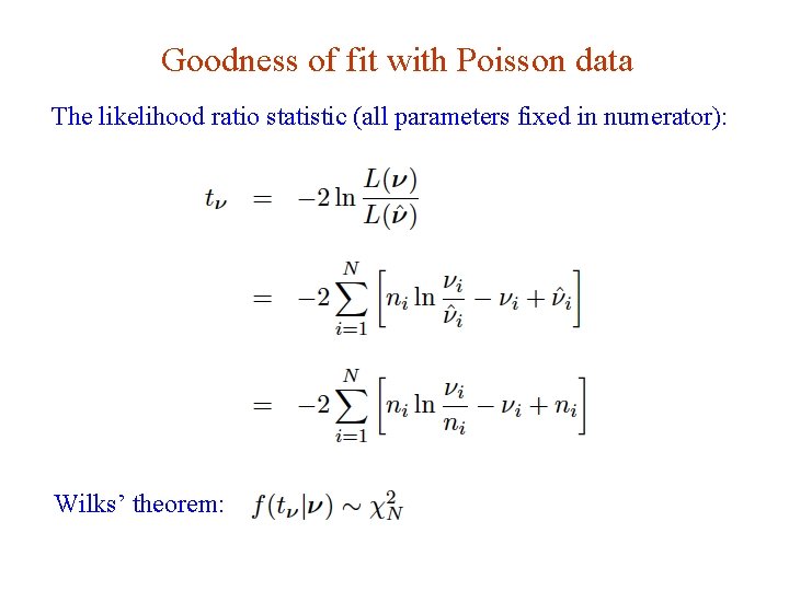
Goodness of fit with Poisson data The likelihood ratio statistic (all parameters fixed in numerator): Wilks’ theorem: G. Cowan INFN School of Statistics, Ischia, 7 -10 May 2017 65

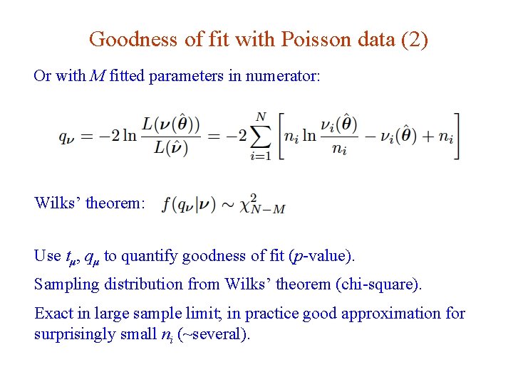
Goodness of fit with Poisson data (2) Or with M fitted parameters in numerator: Wilks’ theorem: Use tμ, qμ to quantify goodness of fit (p-value). Sampling distribution from Wilks’ theorem (chi-square). Exact in large sample limit; in practice good approximation for surprisingly small ni (~several). G. Cowan INFN School of Statistics, Ischia, 7 -10 May 2017 66

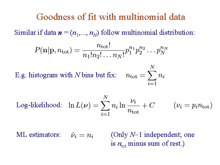
Goodness of fit with multinomial data Similar if data n = (n 1, . . . , nΝ) follow multinomial distribution: E. g. histogram with N bins but fix: Log-likelihood: ML estimators: G. Cowan (Only N-1 independent; one is ntot minus sum of rest. ) INFN School of Statistics, Ischia, 7 -10 May 2017 67

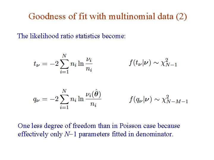
Goodness of fit with multinomial data (2) The likelihood ratio statistics become: One less degree of freedom than in Poisson case because effectively only N-1 parameters fitted in denominator. G. Cowan INFN School of Statistics, Ischia, 7 -10 May 2017 68

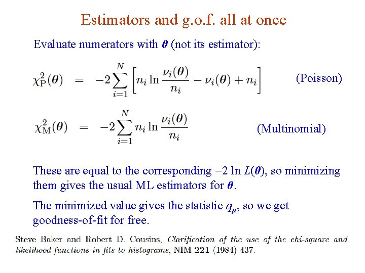
Estimators and g. o. f. all at once Evaluate numerators with θ (not its estimator): (Poisson) (Multinomial) These are equal to the corresponding -2 ln L(θ), so minimizing them gives the usual ML estimators for θ. The minimized value gives the statistic qμ, so we get goodness-of-fit for free. G. Cowan INFN School of Statistics, Ischia, 7 -10 May 2017 69

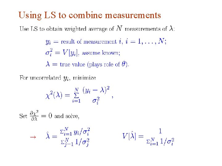
Using LS to combine measurements G. Cowan INFN School of Statistics, Ischia, 7 -10 May 2017 70

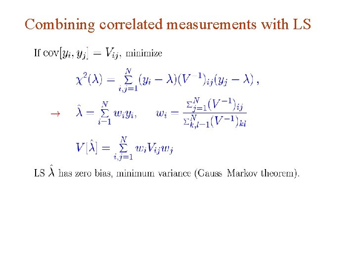
Combining correlated measurements with LS G. Cowan INFN School of Statistics, Ischia, 7 -10 May 2017 71

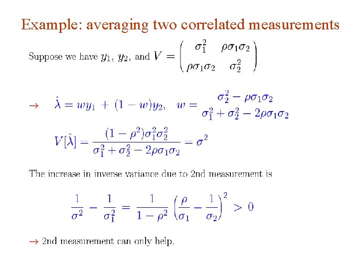
Example: averaging two correlated measurements G. Cowan INFN School of Statistics, Ischia, 7 -10 May 2017 72

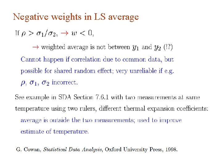
Negative weights in LS average G. Cowan INFN School of Statistics, Ischia, 7 -10 May 2017 73

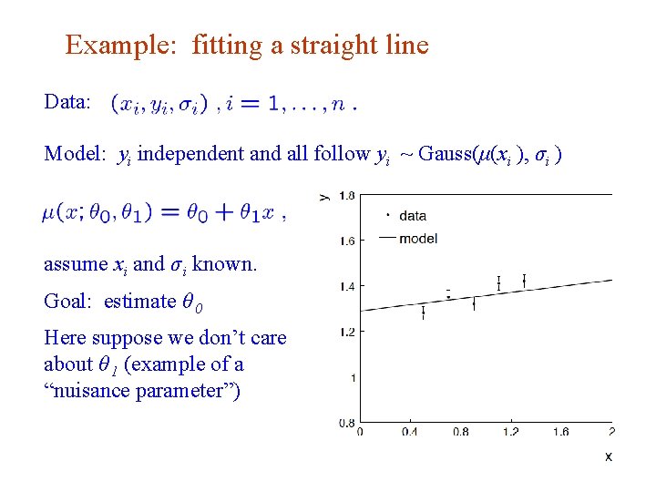
Example: fitting a straight line Data: Model: yi independent and all follow yi ~ Gauss(μ(xi ), σi ) assume xi and σ i known. Goal: estimate θ 0 Here suppose we don’t care about θ 1 (example of a “nuisance parameter”) G. Cowan INFN School of Statistics, Ischia, 7 -10 May 2017 74

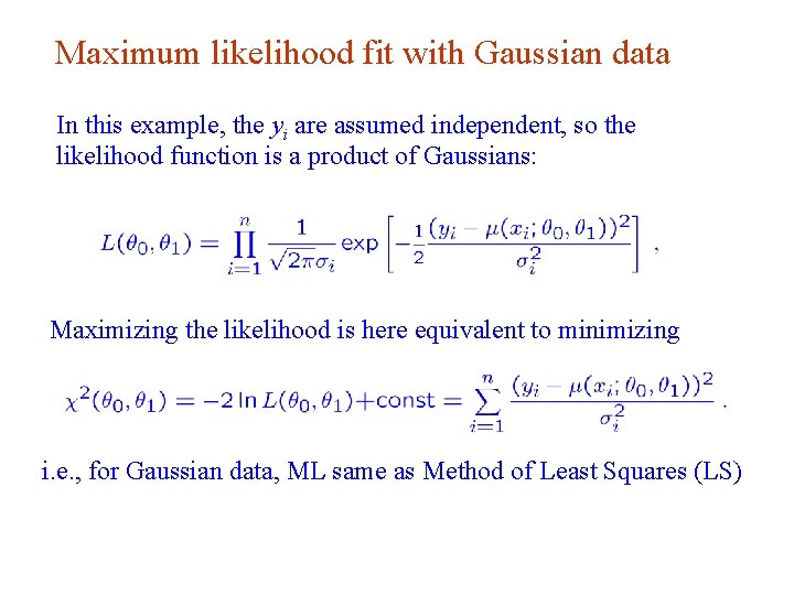
Maximum likelihood fit with Gaussian data In this example, the yi are assumed independent, so the likelihood function is a product of Gaussians: Maximizing the likelihood is here equivalent to minimizing i. e. , for Gaussian data, ML same as Method of Least Squares (LS) G. Cowan INFN School of Statistics, Ischia, 7 -10 May 2017 75

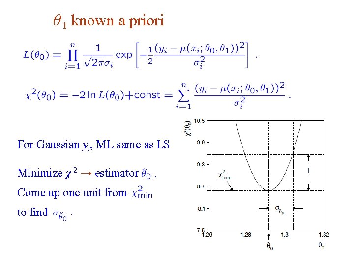
θ 1 known a priori For Gaussian yi, ML same as LS Minimize χ 2 → estimator Come up one unit from to find G. Cowan INFN School of Statistics, Ischia, 7 -10 May 2017 76

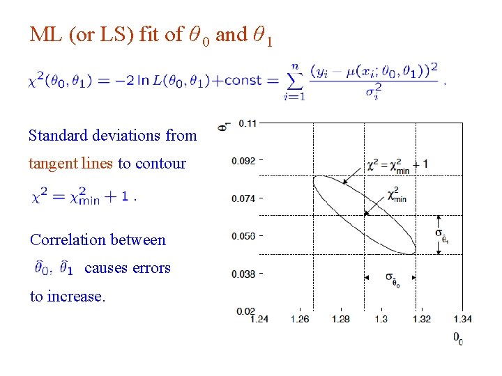
ML (or LS) fit of θ 0 and θ 1 Standard deviations from tangent lines to contour Correlation between causes errors to increase. G. Cowan INFN School of Statistics, Ischia, 7 -10 May 2017 77

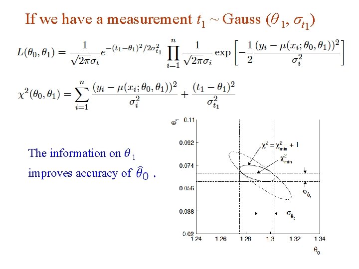
If we have a measurement t 1 ~ Gauss (θ 1, σt 1) The information on θ 1 improves accuracy of G. Cowan INFN School of Statistics, Ischia, 7 -10 May 2017 78

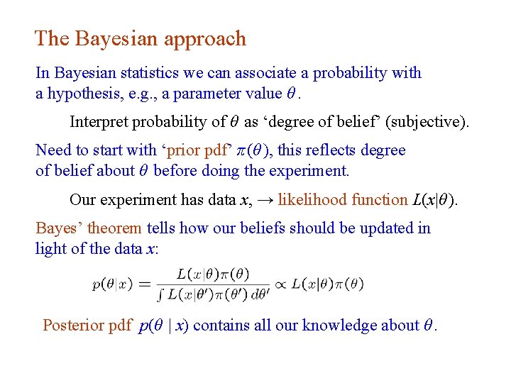
The Bayesian approach In Bayesian statistics we can associate a probability with a hypothesis, e. g. , a parameter value θ. Interpret probability of θ as ‘degree of belief’ (subjective). Need to start with ‘prior pdf’ π (θ ), this reflects degree of belief about θ before doing the experiment. Our experiment has data x, → likelihood function L(x|θ ). Bayes’ theorem tells how our beliefs should be updated in light of the data x: Posterior pdf p(θ | x) contains all our knowledge about θ. G. Cowan INFN School of Statistics, Ischia, 7 -10 May 2017 Lecture 13 page 79

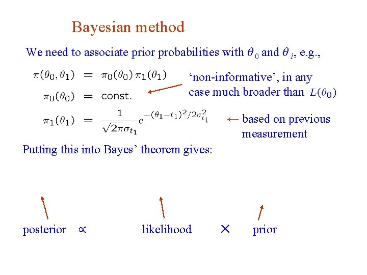
Bayesian method We need to associate prior probabilities with θ 0 and θ 1, e. g. , ‘non-informative’, in any case much broader than ← based on previous measurement Putting this into Bayes’ theorem gives: posterior G. Cowan ∝ likelihood ✕ prior INFN School of Statistics, Ischia, 7 -10 May 2017 80

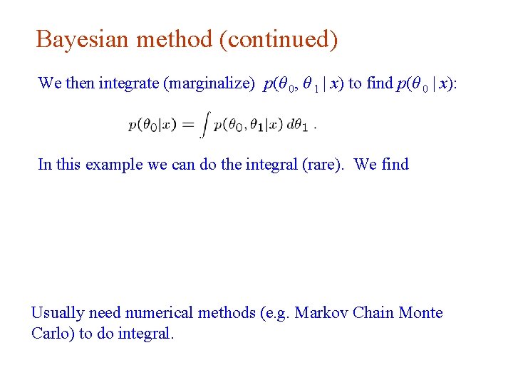
Bayesian method (continued) We then integrate (marginalize) p(θ 0, θ 1 | x) to find p(θ 0 | x): In this example we can do the integral (rare). We find Usually need numerical methods (e. g. Markov Chain Monte Carlo) to do integral. G. Cowan INFN School of Statistics, Ischia, 7 -10 May 2017 81

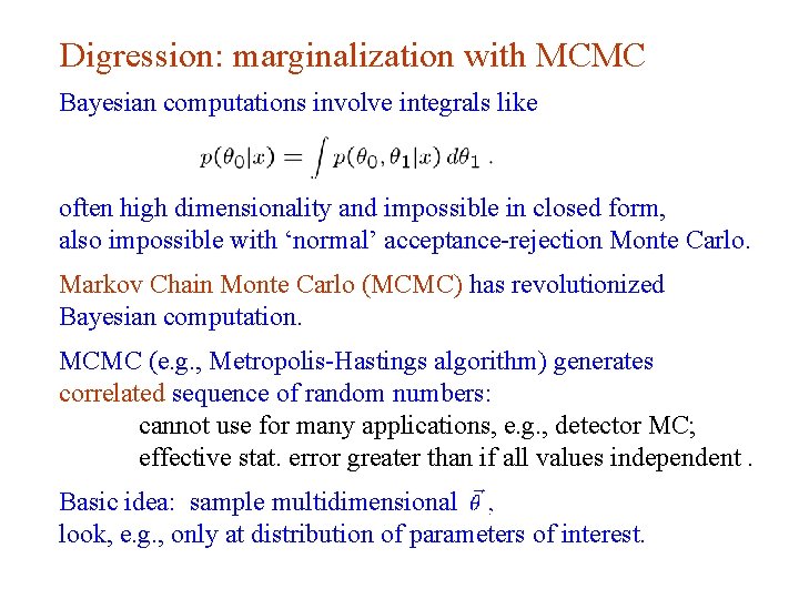
Digression: marginalization with MCMC Bayesian computations involve integrals like often high dimensionality and impossible in closed form, also impossible with ‘normal’ acceptance-rejection Monte Carlo. Markov Chain Monte Carlo (MCMC) has revolutionized Bayesian computation. MCMC (e. g. , Metropolis-Hastings algorithm) generates correlated sequence of random numbers: cannot use for many applications, e. g. , detector MC; effective stat. error greater than if all values independent. Basic idea: sample multidimensional look, e. g. , only at distribution of parameters of interest. G. Cowan INFN School of Statistics, Ischia, 7 -10 May 2017 82

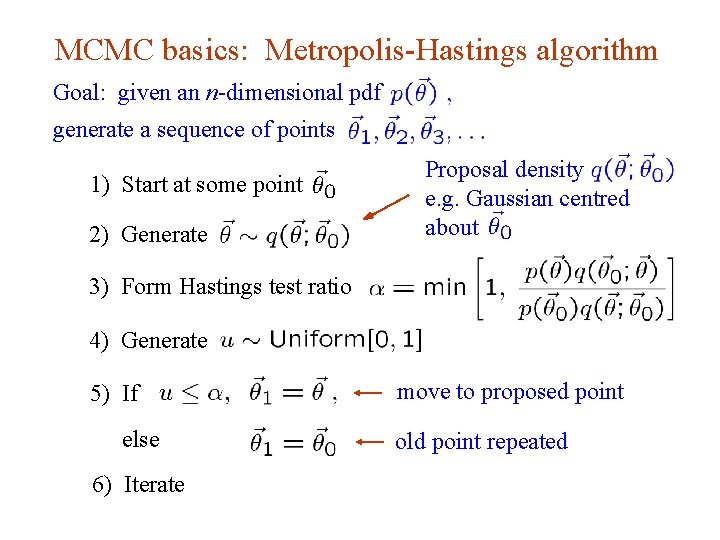
MCMC basics: Metropolis-Hastings algorithm Goal: given an n-dimensional pdf generate a sequence of points 1) Start at some point 2) Generate Proposal density e. g. Gaussian centred about 3) Form Hastings test ratio 4) Generate 5) If else move to proposed point old point repeated 6) Iterate G. Cowan INFN School of Statistics, Ischia, 7 -10 May 2017 83

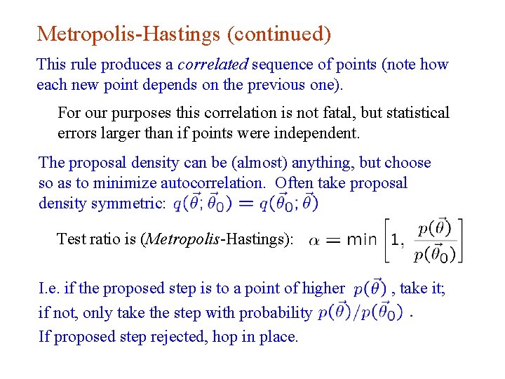
Metropolis-Hastings (continued) This rule produces a correlated sequence of points (note how each new point depends on the previous one). For our purposes this correlation is not fatal, but statistical errors larger than if points were independent. The proposal density can be (almost) anything, but choose so as to minimize autocorrelation. Often take proposal density symmetric: Test ratio is (Metropolis-Hastings): I. e. if the proposed step is to a point of higher if not, only take the step with probability If proposed step rejected, hop in place. G. Cowan INFN School of Statistics, Ischia, 7 -10 May 2017 , take it; 84

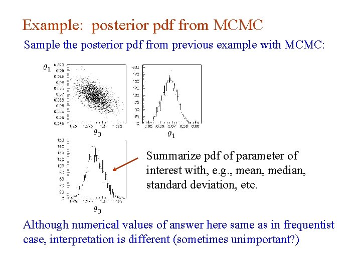
Example: posterior pdf from MCMC Sample the posterior pdf from previous example with MCMC: Summarize pdf of parameter of interest with, e. g. , mean, median, standard deviation, etc. Although numerical values of answer here same as in frequentist case, interpretation is different (sometimes unimportant? ) G. Cowan INFN School of Statistics, Ischia, 7 -10 May 2017 85

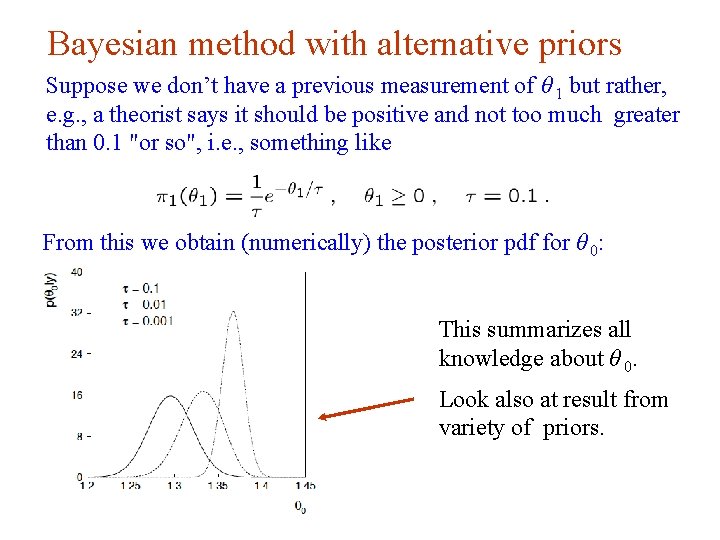
Bayesian method with alternative priors Suppose we don’t have a previous measurement of θ 1 but rather, e. g. , a theorist says it should be positive and not too much greater than 0. 1 "or so", i. e. , something like From this we obtain (numerically) the posterior pdf for θ 0: This summarizes all knowledge about θ 0. Look also at result from variety of priors. G. Cowan INFN School of Statistics, Ischia, 7 -10 May 2017 86

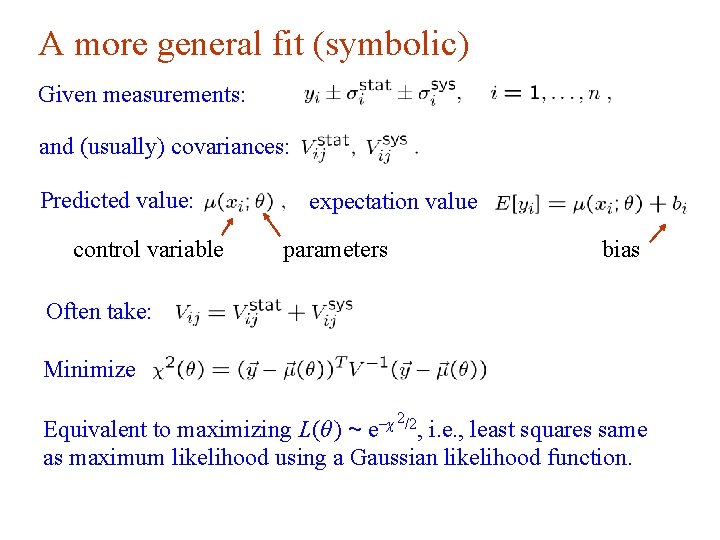
A more general fit (symbolic) Given measurements: and (usually) covariances: Predicted value: expectation value control variable parameters bias Often take: Minimize 2/2 -χ e , Equivalent to maximizing L(θ ) ~ i. e. , least squares same as maximum likelihood using a Gaussian likelihood function. G. Cowan INFN School of Statistics, Ischia, 7 -10 May 2017 87

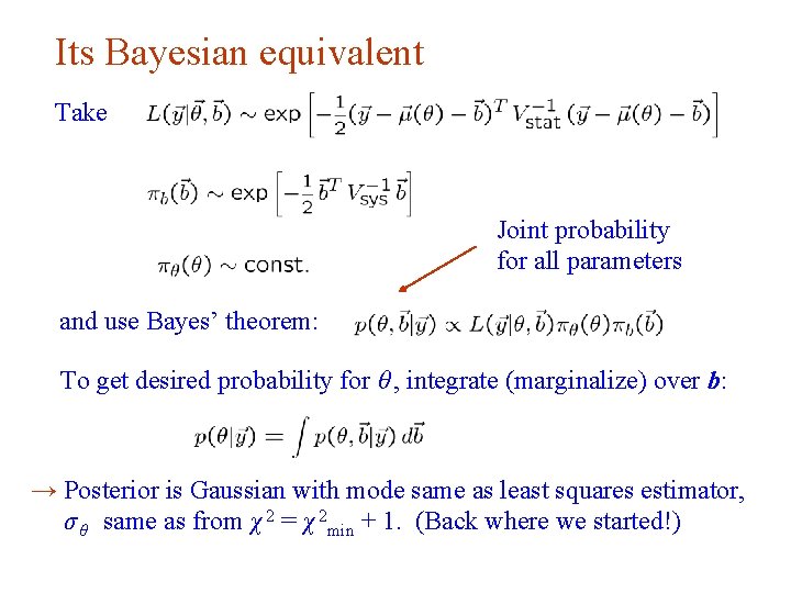
Its Bayesian equivalent Take Joint probability for all parameters and use Bayes’ theorem: To get desired probability for θ , integrate (marginalize) over b: → Posterior is Gaussian with mode same as least squares estimator, σ θ same as from χ 2 = χ 2 min + 1. (Back where we started!) G. Cowan INFN School of Statistics, Ischia, 7 -10 May 2017 88

The error on the error Some systematic errors are well determined Error from finite Monte Carlo sample Some are less obvious Do analysis in n ‘equally valid’ ways and extract systematic error from ‘spread’ in results. Some are educated guesses Guess possible size of missing terms in perturbation series; vary renormalization scale Can we incorporate the ‘error on the error’? (cf. G. D’Agostini 1999; Dose & von der Linden 1999) G. Cowan INFN School of Statistics, Ischia, 7 -10 May 2017 89

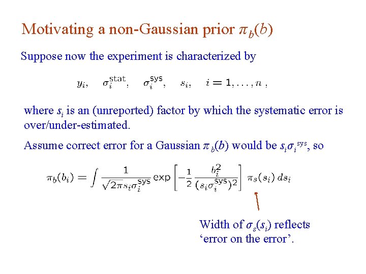
Motivating a non-Gaussian prior π b(b) Suppose now the experiment is characterized by where si is an (unreported) factor by which the systematic error is over/under-estimated. Assume correct error for a Gaussian π b(b) would be siσ isys, so Width of σ s(si) reflects ‘error on the error’. G. Cowan INFN School of Statistics, Ischia, 7 -10 May 2017 90

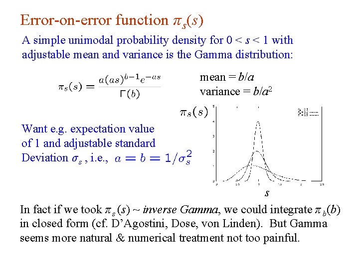
Error-on-error function π s(s) A simple unimodal probability density for 0 < s < 1 with adjustable mean and variance is the Gamma distribution: mean = b/a variance = b/a 2 Want e. g. expectation value of 1 and adjustable standard Deviation σ s , i. e. , s In fact if we took π s (s) ~ inverse Gamma, we could integrate π b(b) in closed form (cf. D’Agostini, Dose, von Linden). But Gamma seems more natural & numerical treatment not too painful. G. Cowan INFN School of Statistics, Ischia, 7 -10 May 2017 91

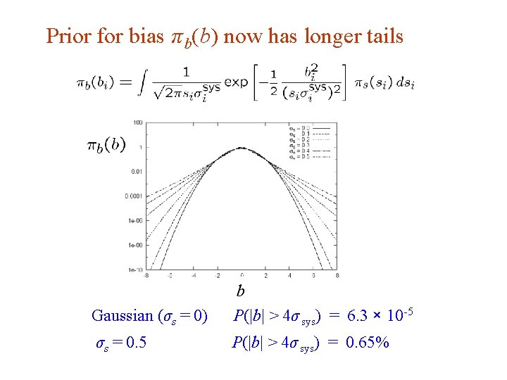
Prior for bias π b(b) now has longer tails G. Cowan Gaussian (σs = 0) b P(|b| > 4σ sys) = 6. 3 × 10 -5 σs = 0. 5 P(|b| > 4σ sys) = 0. 65% INFN School of Statistics, Ischia, 7 -10 May 2017 92

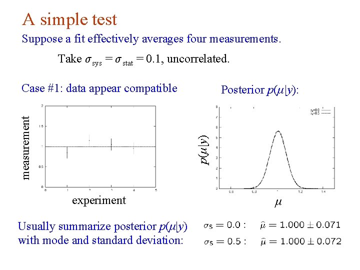
A simple test Suppose a fit effectively averages four measurements. Take σ sys = σ stat = 0. 1, uncorrelated. Posterior p(μ|y): p(μ|y) measurement Case #1: data appear compatible experiment μ Usually summarize posterior p(μ|y) with mode and standard deviation: G. Cowan INFN School of Statistics, Ischia, 7 -10 May 2017 93

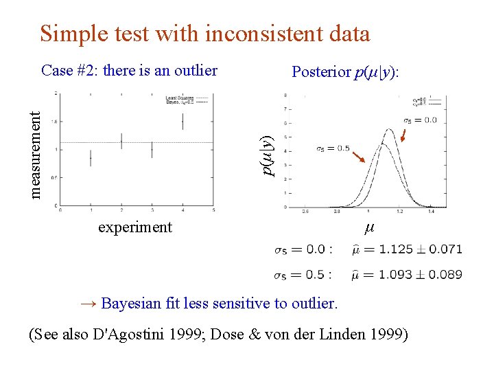
Simple test with inconsistent data Posterior p(μ|y): p(μ|y) measurement Case #2: there is an outlier experiment μ → Bayesian fit less sensitive to outlier. (See also D'Agostini 1999; Dose & von der Linden 1999) G. Cowan INFN School of Statistics, Ischia, 7 -10 May 2017 94

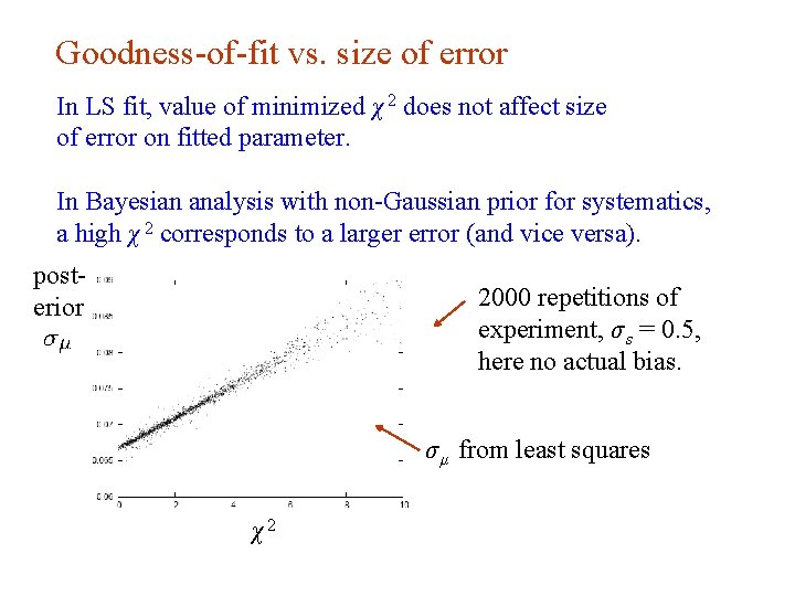
Goodness-of-fit vs. size of error In LS fit, value of minimized χ 2 does not affect size of error on fitted parameter. In Bayesian analysis with non-Gaussian prior for systematics, a high χ 2 corresponds to a larger error (and vice versa). posterior 2000 repetitions of experiment, σ s = 0. 5, here no actual bias. σ μ from least squares χ2 G. Cowan INFN School of Statistics, Ischia, 7 -10 May 2017 95

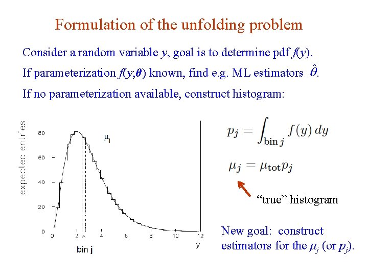
Formulation of the unfolding problem Consider a random variable y, goal is to determine pdf f(y). If parameterization f(y; θ) known, find e. g. ML estimators . If no parameterization available, construct histogram: “true” histogram New goal: construct estimators for the μj (or pj). G. Cowan INFN School of Statistics, Ischia, 7 -10 May 2017 96

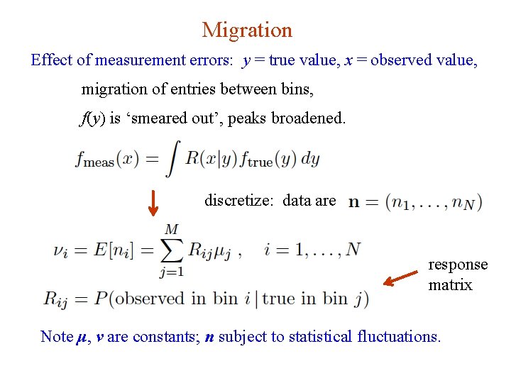
Migration Effect of measurement errors: y = true value, x = observed value, migration of entries between bins, f(y) is ‘smeared out’, peaks broadened. discretize: data are response matrix Note μ, ν are constants; n subject to statistical fluctuations. G. Cowan INFN School of Statistics, Ischia, 7 -10 May 2017 97

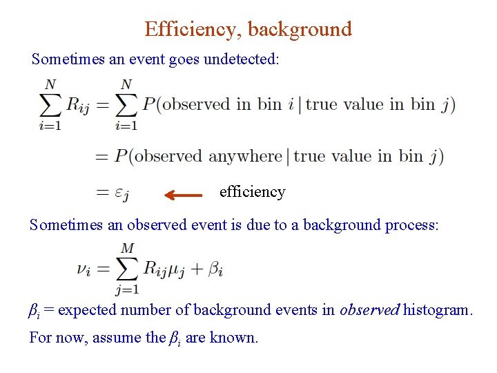
Efficiency, background Sometimes an event goes undetected: efficiency Sometimes an observed event is due to a background process: βi = expected number of background events in observed histogram. For now, assume the βi are known. G. Cowan INFN School of Statistics, Ischia, 7 -10 May 2017 98

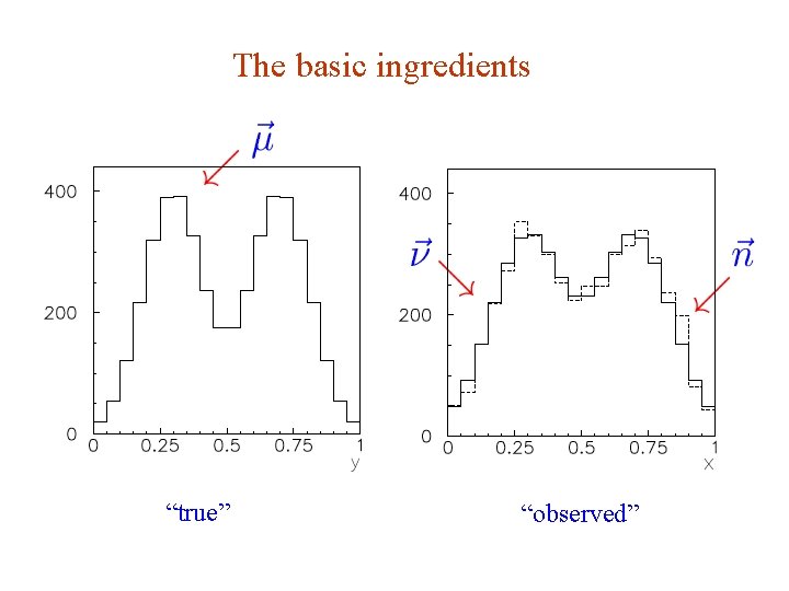
The basic ingredients “true” G. Cowan “observed” INFN School of Statistics, Ischia, 7 -10 May 2017 99

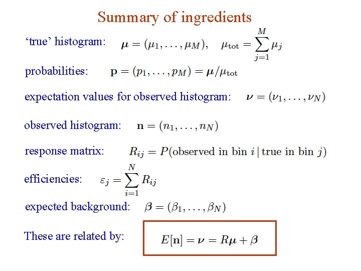
Summary of ingredients ‘true’ histogram: probabilities: expectation values for observed histogram: response matrix: efficiencies: expected background: These are related by: G. Cowan INFN School of Statistics, Ischia, 7 -10 May 2017 100

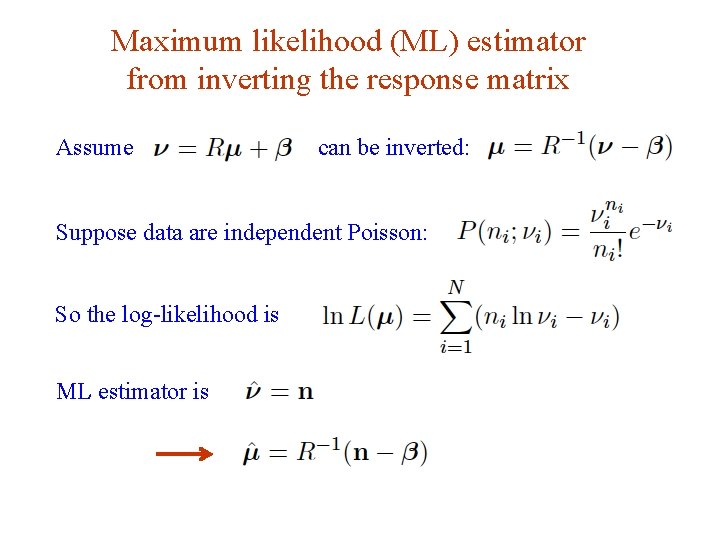
Maximum likelihood (ML) estimator from inverting the response matrix Assume can be inverted: Suppose data are independent Poisson: So the log-likelihood is ML estimator is G. Cowan INFN School of Statistics, Ischia, 7 -10 May 2017 101

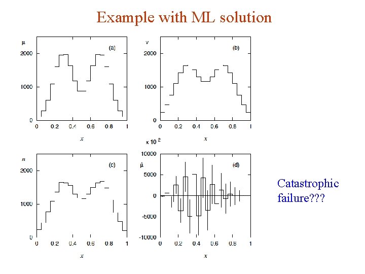
Example with ML solution Catastrophic failure? ? ? G. Cowan INFN School of Statistics, Ischia, 7 -10 May 2017 102

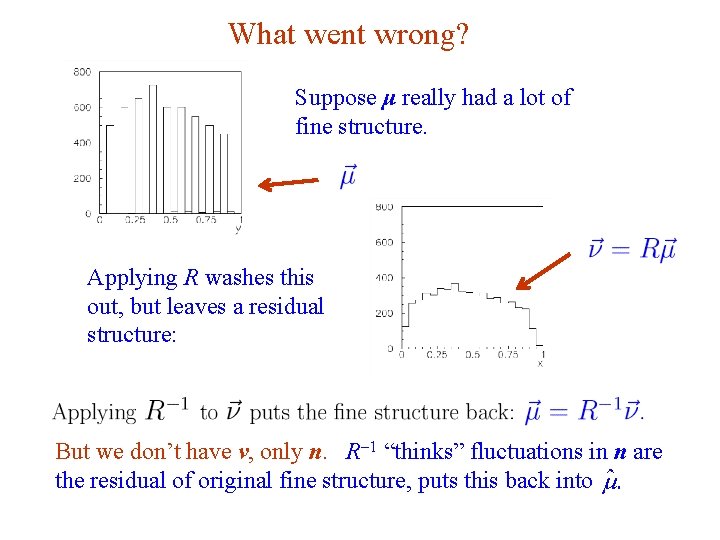
What went wrong? Suppose μ really had a lot of fine structure. Applying R washes this out, but leaves a residual structure: But we don’t have ν, only n. R-1 “thinks” fluctuations in n are the residual of original fine structure, puts this back into G. Cowan INFN School of Statistics, Ischia, 7 -10 May 2017 103

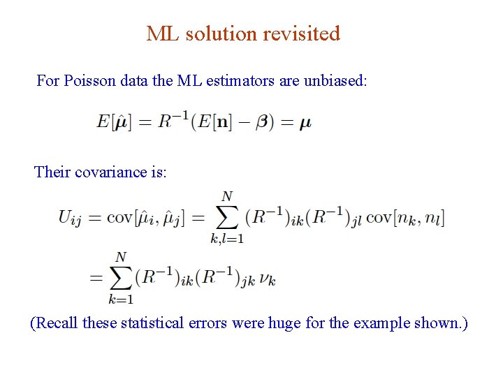
ML solution revisited For Poisson data the ML estimators are unbiased: Their covariance is: (Recall these statistical errors were huge for the example shown. ) G. Cowan INFN School of Statistics, Ischia, 7 -10 May 2017 104

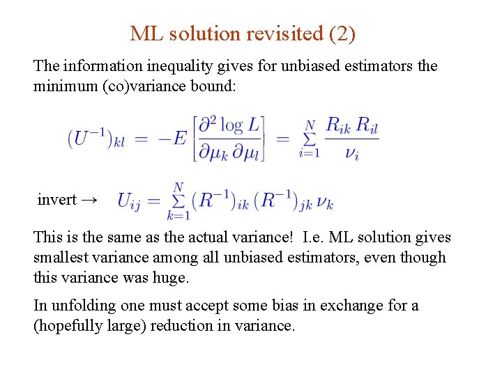
ML solution revisited (2) The information inequality gives for unbiased estimators the minimum (co)variance bound: invert → This is the same as the actual variance! I. e. ML solution gives smallest variance among all unbiased estimators, even though this variance was huge. In unfolding one must accept some bias in exchange for a (hopefully large) reduction in variance. G. Cowan INFN School of Statistics, Ischia, 7 -10 May 2017 105

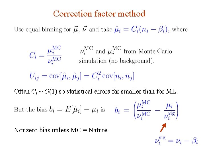
Correction factor method Often Ci ~ O(1) so statistical errors far smaller than for ML. Nonzero bias unless MC = Nature. G. Cowan INFN School of Statistics, Ischia, 7 -10 May 2017 106

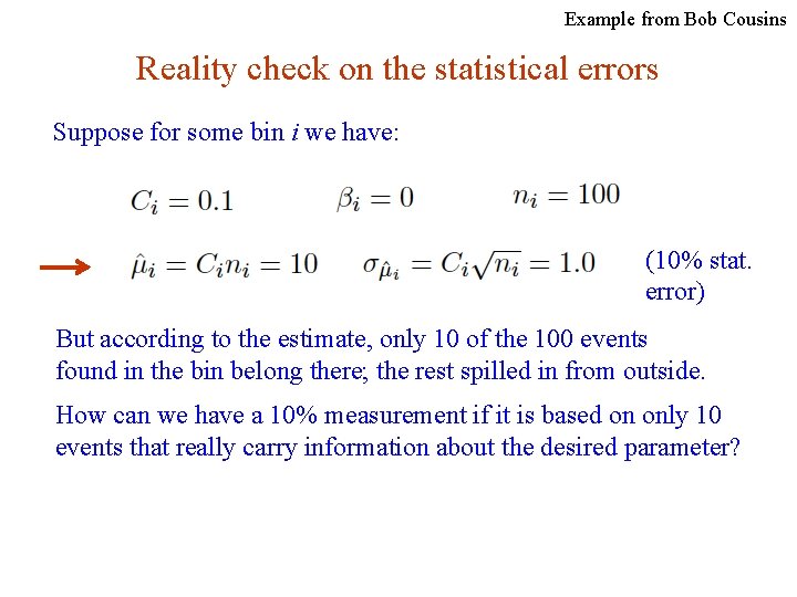
Example from Bob Cousins Reality check on the statistical errors Suppose for some bin i we have: (10% stat. error) But according to the estimate, only 10 of the 100 events found in the bin belong there; the rest spilled in from outside. How can we have a 10% measurement if it is based on only 10 events that really carry information about the desired parameter? G. Cowan INFN School of Statistics, Ischia, 7 -10 May 2017 107

Discussion of correction factor method As with all unfolding methods, we get a reduction in statistical error in exchange for a bias; here the bias is difficult to quantify (difficult also for many other unfolding methods). The bias should be small if the bin width is substantially larger than the resolution, so that there is not much bin migration. So if other uncertainties dominate in an analysis, correction factors may provide a quick and simple solution (a “first-look”). Still the method has important flaws and it would be best to avoid it. G. Cowan INFN School of Statistics, Ischia, 7 -10 May 2017 108

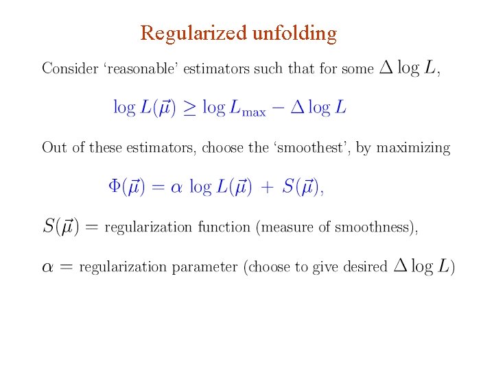
Regularized unfolding G. Cowan INFN School of Statistics, Ischia, 7 -10 May 2017 109

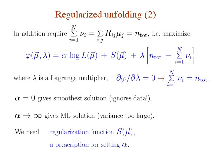
Regularized unfolding (2) G. Cowan INFN School of Statistics, Ischia, 7 -10 May 2017 110

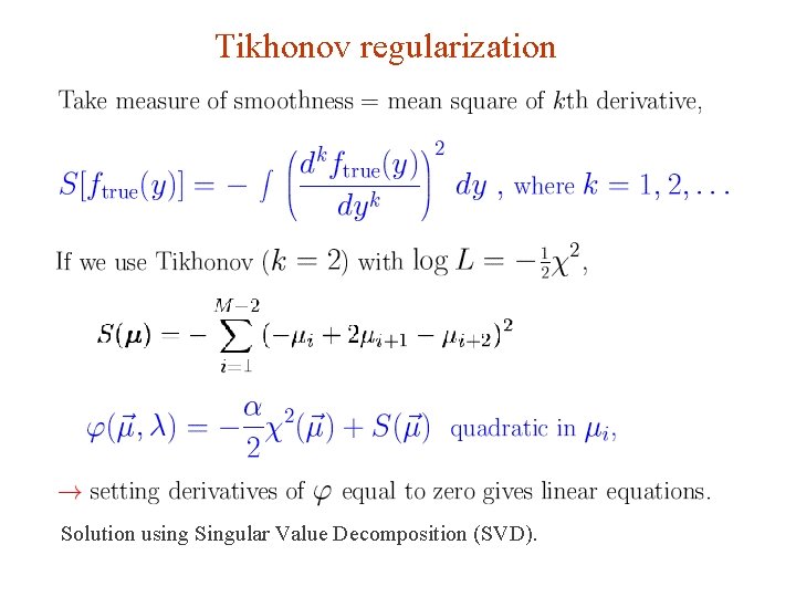
Tikhonov regularization Solution using Singular Value Decomposition (SVD). G. Cowan INFN School of Statistics, Ischia, 7 -10 May 2017 111

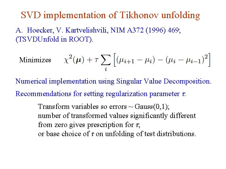
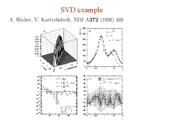
SVD implementation of Tikhonov unfolding A. Hoecker, V. Kartvelishvili, NIM A 372 (1996) 469; (TSVDUnfold in ROOT). Minimizes Numerical implementation using Singular Value Decomposition. Recommendations for setting regularization parameter τ: Transform variables so errors ~ Gauss(0, 1); number of transformed values significantly different from zero gives prescription for τ; or base choice of τ on unfolding of test distributions. G. Cowan INFN School of Statistics, Ischia, 7 -10 May 2017 112

SVD example G. Cowan INFN School of Statistics, Ischia, 7 -10 May 2017 113

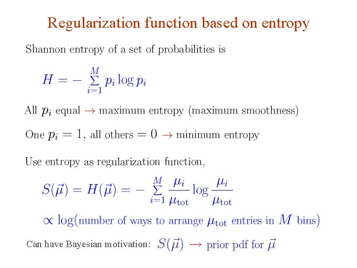
Regularization function based on entropy Can have Bayesian motivation: G. Cowan INFN School of Statistics, Ischia, 7 -10 May 2017 114

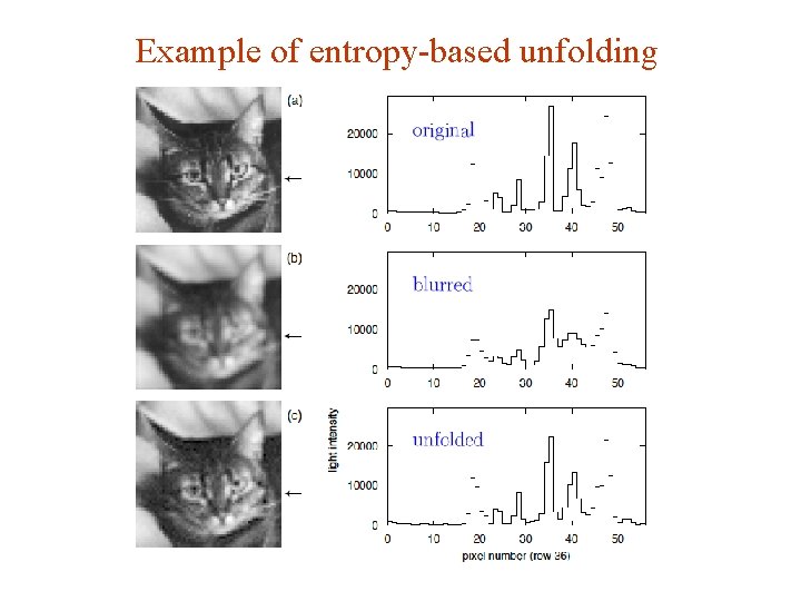
Example of entropy-based unfolding G. Cowan INFN School of Statistics, Ischia, 7 -10 May 2017 115

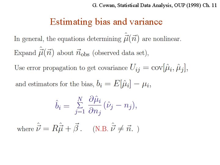
G. Cowan, Statistical Data Analysis, OUP (1998) Ch. 11 Estimating bias and variance G. Cowan INFN School of Statistics, Ischia, 7 -10 May 2017 116

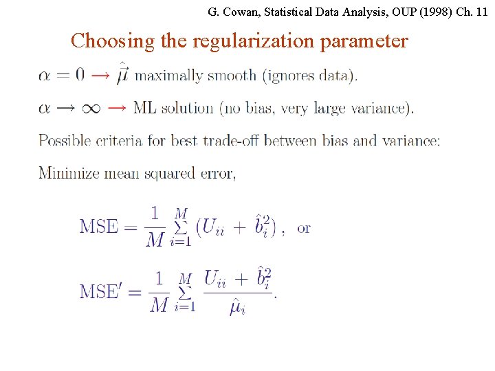
G. Cowan, Statistical Data Analysis, OUP (1998) Ch. 11 Choosing the regularization parameter G. Cowan INFN School of Statistics, Ischia, 7 -10 May 2017 117

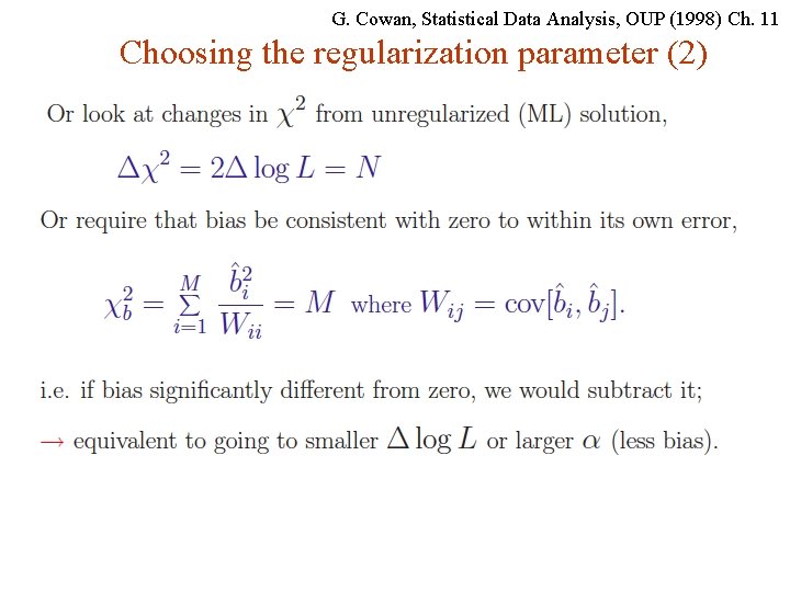
G. Cowan, Statistical Data Analysis, OUP (1998) Ch. 11 Choosing the regularization parameter (2) G. Cowan INFN School of Statistics, Ischia, 7 -10 May 2017 118

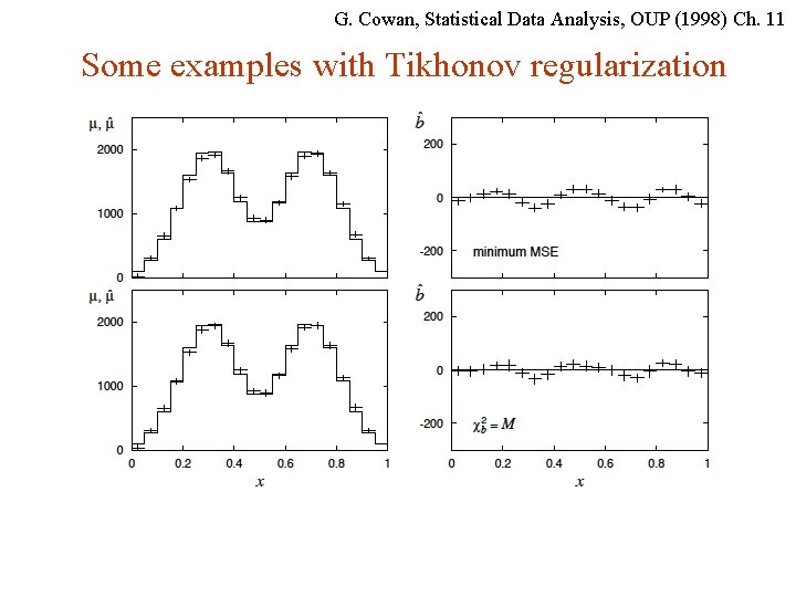
G. Cowan, Statistical Data Analysis, OUP (1998) Ch. 11 Some examples with Tikhonov regularization G. Cowan INFN School of Statistics, Ischia, 7 -10 May 2017 119

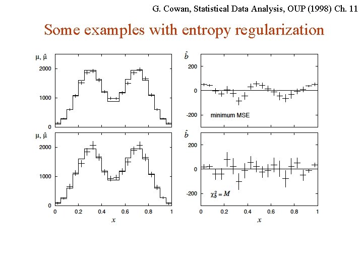
G. Cowan, Statistical Data Analysis, OUP (1998) Ch. 11 Some examples with entropy regularization G. Cowan INFN School of Statistics, Ischia, 7 -10 May 2017 120

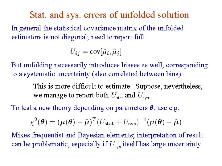
Stat. and sys. errors of unfolded solution In general the statistical covariance matrix of the unfolded estimators is not diagonal; need to report full But unfolding necessarily introduces biases as well, corresponding to a systematic uncertainty (also correlated between bins). This is more difficult to estimate. Suppose, nevertheless, we manage to report both Ustat and Usys. To test a new theory depending on parameters θ, use e. g. Mixes frequentist and Bayesian elements; interpretation of result can be problematic, especially if Usys itself has large uncertainty. G. Cowan INFN School of Statistics, Ischia, 7 -10 May 2017 121

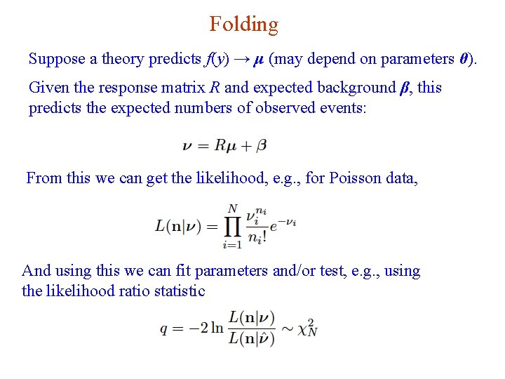
Folding Suppose a theory predicts f(y) → μ (may depend on parameters θ). Given the response matrix R and expected background β, this predicts the expected numbers of observed events: From this we can get the likelihood, e. g. , for Poisson data, And using this we can fit parameters and/or test, e. g. , using the likelihood ratio statistic G. Cowan INFN School of Statistics, Ischia, 7 -10 May 2017 122

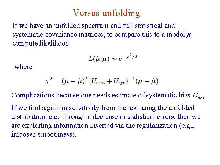
Versus unfolding If we have an unfolded spectrum and full statistical and systematic covariance matrices, to compare this to a model μ compute likelihood where Complications because one needs estimate of systematic bias Usys. If we find a gain in sensitivity from the test using the unfolded distribution, e. g. , through a decrease in statistical errors, then we are exploiting information inserted via the regularization (e. g. , imposed smoothness). G. Cowan INFN School of Statistics, Ischia, 7 -10 May 2017 123

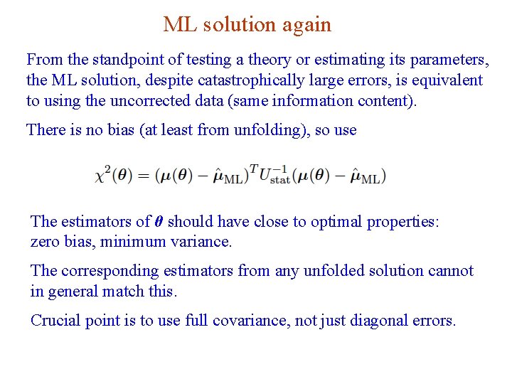
ML solution again From the standpoint of testing a theory or estimating its parameters, the ML solution, despite catastrophically large errors, is equivalent to using the uncorrected data (same information content). There is no bias (at least from unfolding), so use The estimators of θ should have close to optimal properties: zero bias, minimum variance. The corresponding estimators from any unfolded solution cannot in general match this. Crucial point is to use full covariance, not just diagonal errors. G. Cowan INFN School of Statistics, Ischia, 7 -10 May 2017 124

Summary/discussion Unfolding can be a minefield and is not necessary if goal is to compare measured distribution with a model prediction. Even comparison of uncorrected distribution with future theories not a problem, as long as it is reported together with the expected background and response matrix. In practice complications because these ingredients have uncertainties, and they must be reported as well. Unfolding useful for getting an actual estimate of the distribution we think we’ve measured; can e. g. compare ATLAS/CMS. Model test using unfolded distribution should take account of the (correlated) bias introduced by the unfolding procedure. G. Cowan INFN School of Statistics, Ischia, 7 -10 May 2017 125

Finally. . . Estimation of parameters is usually the “easy” part of statistics: Frequentist: maximize the likelihood. Bayesian: find posterior pdf and summarize (e. g. mode). Standard tools for quantifying precision of estimates: Variance of estimators, confidence intervals, . . . But there are many potential stumbling blocks: bias versus variance trade-off (how many parameters to fit? ); goodness of fit (usually only for LS or binned data); choice of prior for Bayesian approach; unexpected behaviour in LS averages with correlations, . . . We can practice this later with MINUIT. G. Cowan INFN School of Statistics, Ischia, 7 -10 May 2017 126

Extra Slides G. Cowan INFN School of Statistics, Ischia, 7 -10 May 2017 127

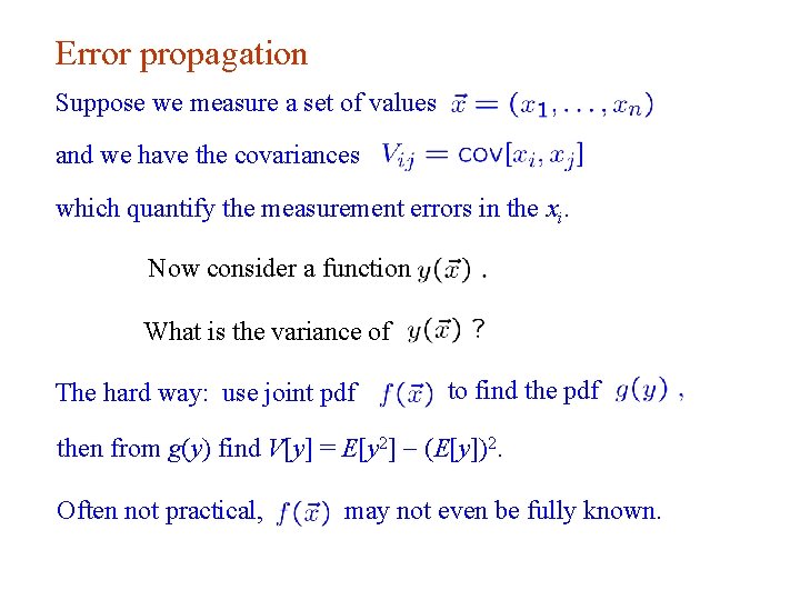
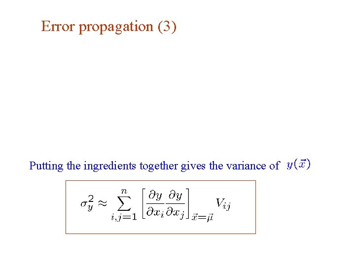
Error propagation Suppose we measure a set of values and we have the covariances which quantify the measurement errors in the xi. Now consider a function What is the variance of The hard way: use joint pdf to find the pdf then from g(y) find V[y] = E[y 2] - (E[y])2. Often not practical, G. Cowan may not even be fully known. INFN School of Statistics, Ischia, 7 -10 May 2017 128

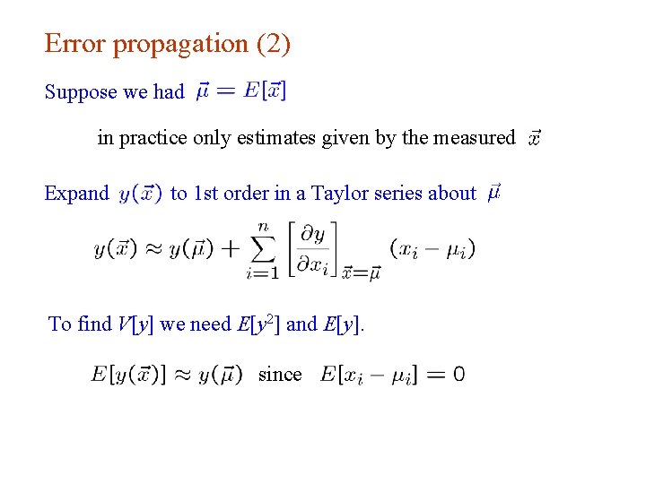
Error propagation (2) Suppose we had in practice only estimates given by the measured Expand to 1 st order in a Taylor series about To find V[y] we need E[y 2] and E[y]. since G. Cowan INFN School of Statistics, Ischia, 7 -10 May 2017 129

Error propagation (3) Putting the ingredients together gives the variance of G. Cowan INFN School of Statistics, Ischia, 7 -10 May 2017 130

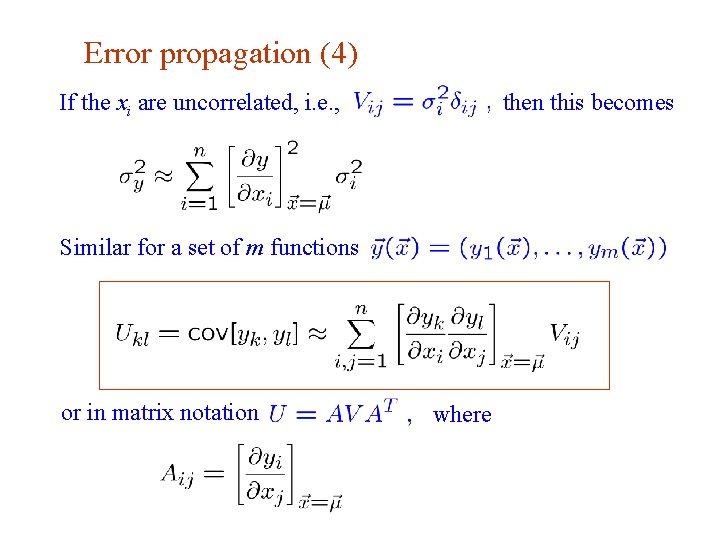
Error propagation (4) If the xi are uncorrelated, i. e. , then this becomes Similar for a set of m functions or in matrix notation G. Cowan where INFN School of Statistics, Ischia, 7 -10 May 2017 131

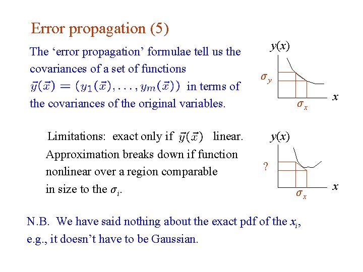
Error propagation (5) The ‘error propagation’ formulae tell us the covariances of a set of functions in terms of the covariances of the original variables. Limitations: exact only if linear. Approximation breaks down if function nonlinear over a region comparable in size to the σ i. y(x) σy σx x y(x) ? σx x N. B. We have said nothing about the exact pdf of the xi, e. g. , it doesn’t have to be Gaussian. G. Cowan INFN School of Statistics, Ischia, 7 -10 May 2017 132

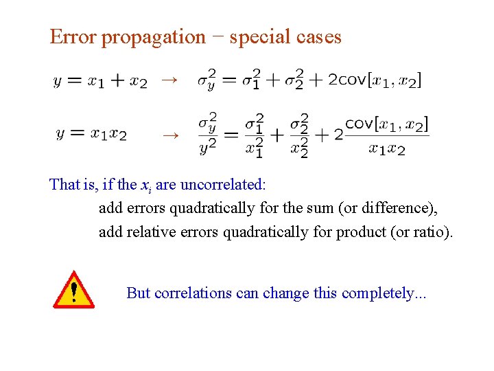
Error propagation − special cases → → That is, if the xi are uncorrelated: add errors quadratically for the sum (or difference), add relative errors quadratically for product (or ratio). But correlations can change this completely. . . G. Cowan INFN School of Statistics, Ischia, 7 -10 May 2017 133

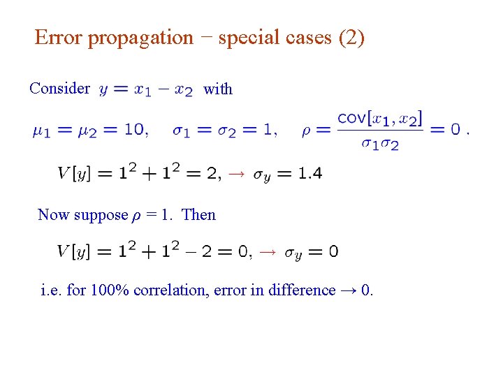
Error propagation − special cases (2) Consider with Now suppose ρ = 1. Then i. e. for 100% correlation, error in difference → 0. G. Cowan INFN School of Statistics, Ischia, 7 -10 May 2017 134

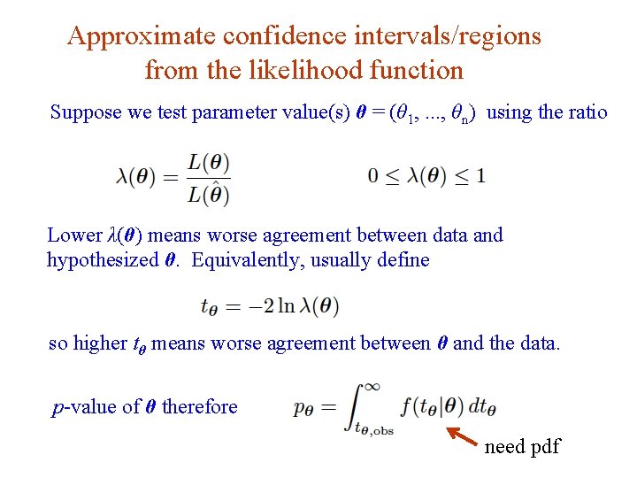
Approximate confidence intervals/regions from the likelihood function Suppose we test parameter value(s) θ = (θ 1, . . . , θn) using the ratio Lower λ(θ) means worse agreement between data and hypothesized θ. Equivalently, usually define so higher tθ means worse agreement between θ and the data. p-value of θ therefore G. Cowan INFN School of Statistics, Ischia, 7 -10 May 2017 need pdf 135

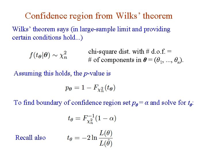
Confidence region from Wilks’ theorem says (in large-sample limit and providing certain conditions hold. . . ) chi-square dist. with # d. o. f. = # of components in θ = (θ 1, . . . , θn). Assuming this holds, the p-value is To find boundary of confidence region set pθ = α and solve for tθ: Recall also G. Cowan INFN School of Statistics, Ischia, 7 -10 May 2017 136

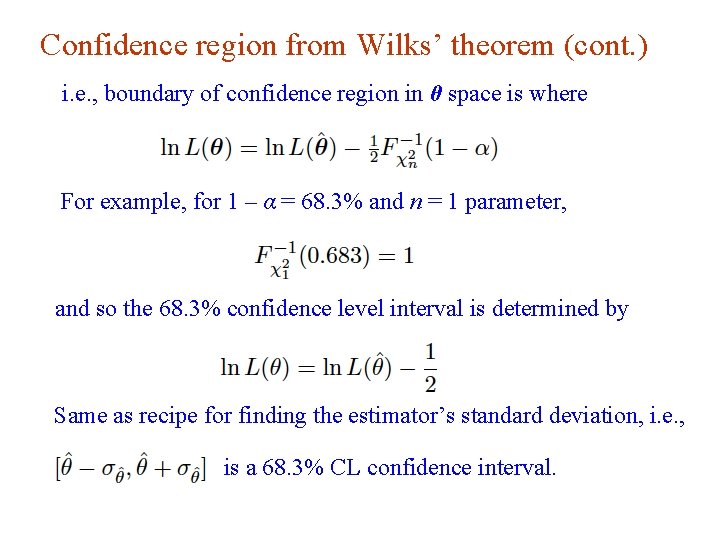
Confidence region from Wilks’ theorem (cont. ) i. e. , boundary of confidence region in θ space is where For example, for 1 – α = 68. 3% and n = 1 parameter, and so the 68. 3% confidence level interval is determined by Same as recipe for finding the estimator’s standard deviation, i. e. , is a 68. 3% CL confidence interval. G. Cowan INFN School of Statistics, Ischia, 7 -10 May 2017 137

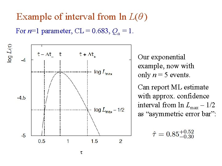
Example of interval from ln L(θ ) For n=1 parameter, CL = 0. 683, Qα = 1. Our exponential example, now with only n = 5 events. Can report ML estimate with approx. confidence interval from ln Lmax – 1/2 as “asymmetric error bar”: G. Cowan INFN School of Statistics, Ischia, 7 -10 May 2017 138

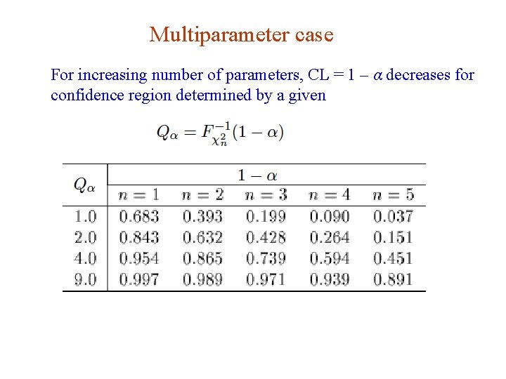
Multiparameter case For increasing number of parameters, CL = 1 – α decreases for confidence region determined by a given G. Cowan INFN School of Statistics, Ischia, 7 -10 May 2017 139

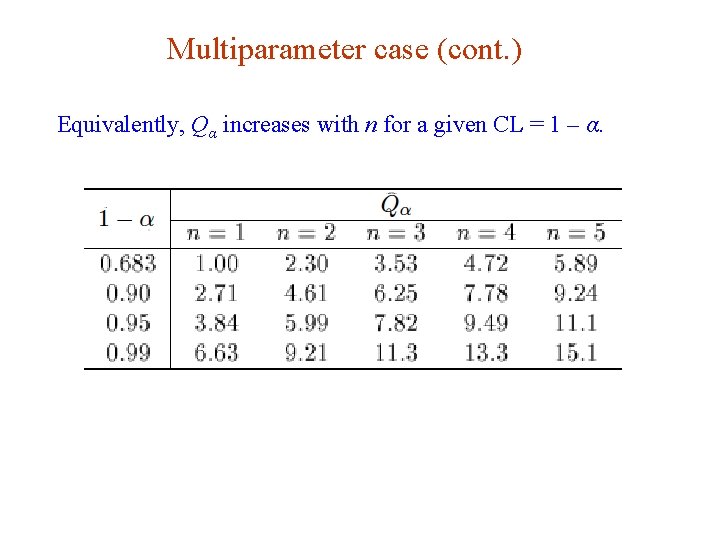
Multiparameter case (cont. ) Equivalently, Qα increases with n for a given CL = 1 – α. G. Cowan INFN School of Statistics, Ischia, 7 -10 May 2017 140

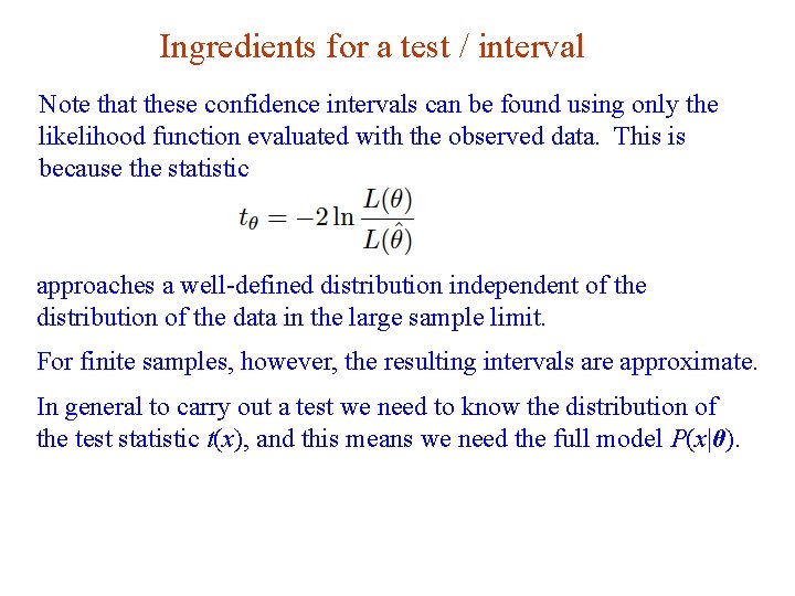
Ingredients for a test / interval Note that these confidence intervals can be found using only the likelihood function evaluated with the observed data. This is because the statistic approaches a well-defined distribution independent of the distribution of the data in the large sample limit. For finite samples, however, the resulting intervals are approximate. In general to carry out a test we need to know the distribution of the test statistic t(x), and this means we need the full model P(x|θ). G. Cowan INFN School of Statistics, Ischia, 7 -10 May 2017 141

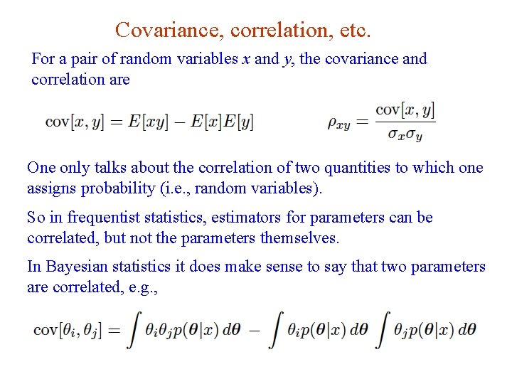
Covariance, correlation, etc. For a pair of random variables x and y, the covariance and correlation are One only talks about the correlation of two quantities to which one assigns probability (i. e. , random variables). So in frequentist statistics, estimators for parameters can be correlated, but not the parameters themselves. In Bayesian statistics it does make sense to say that two parameters are correlated, e. g. , G. Cowan INFN School of Statistics, Ischia, 7 -10 May 2017 142

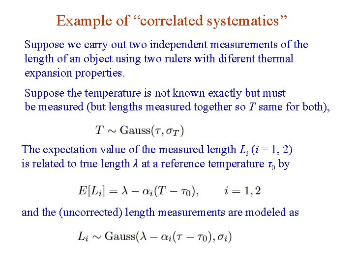
Example of “correlated systematics” Suppose we carry out two independent measurements of the length of an object using two rulers with diferent thermal expansion properties. Suppose the temperature is not known exactly but must be measured (but lengths measured together so T same for both), The expectation value of the measured length Li (i = 1, 2) is related to true length λ at a reference temperature τ0 by and the (uncorrected) length measurements are modeled as G. Cowan INFN School of Statistics, Ischia, 7 -10 May 2017 143

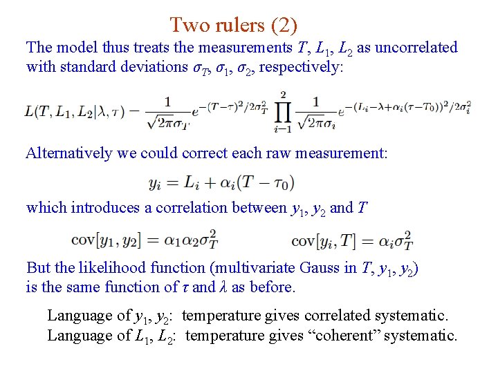
Two rulers (2) The model thus treats the measurements T, L 1, L 2 as uncorrelated with standard deviations σT, σ1, σ2, respectively: Alternatively we could correct each raw measurement: which introduces a correlation between y 1, y 2 and T But the likelihood function (multivariate Gauss in T, y 1, y 2) is the same function of τ and λ as before. Language of y 1, y 2: temperature gives correlated systematic. Language of L 1, L 2: temperature gives “coherent” systematic. G. Cowan INFN School of Statistics, Ischia, 7 -10 May 2017 144

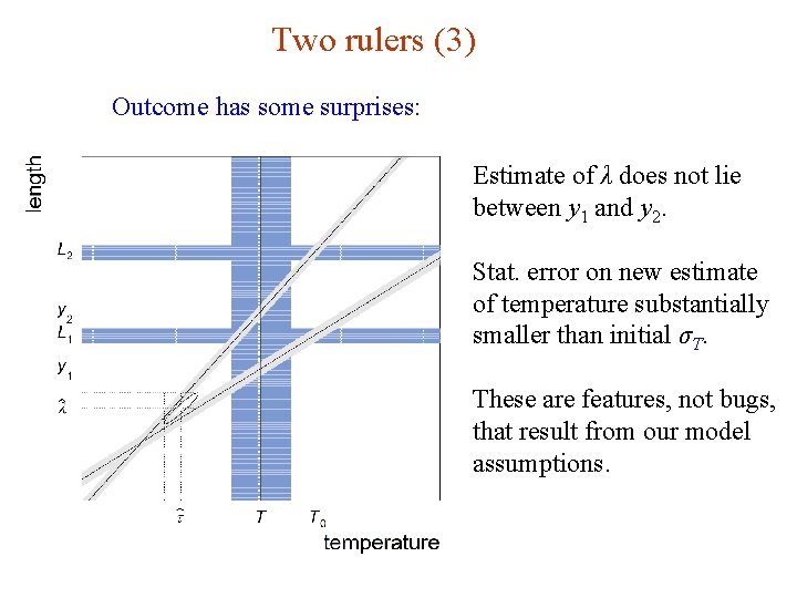
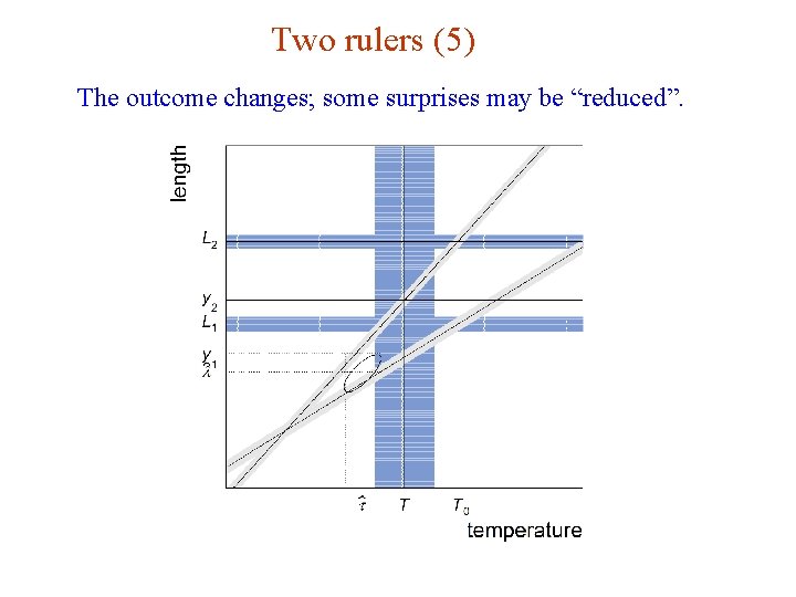
Two rulers (3) Outcome has some surprises: Estimate of λ does not lie between y 1 and y 2. Stat. error on new estimate of temperature substantially smaller than initial σT. These are features, not bugs, that result from our model assumptions. G. Cowan INFN School of Statistics, Ischia, 7 -10 May 2017 145

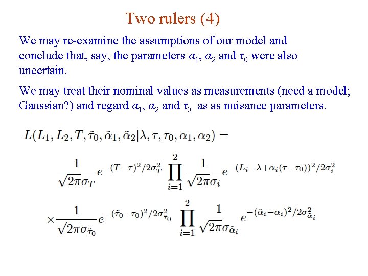
Two rulers (4) We may re-examine the assumptions of our model and conclude that, say, the parameters α 1, α 2 and τ0 were also uncertain. We may treat their nominal values as measurements (need a model; Gaussian? ) and regard α 1, α 2 and τ0 as as nuisance parameters. G. Cowan INFN School of Statistics, Ischia, 7 -10 May 2017 146

Two rulers (5) The outcome changes; some surprises may be “reduced”. G. Cowan INFN School of Statistics, Ischia, 7 -10 May 2017 147